Term Structures

QuantLib provides a module for the representation of different term structures used in Quantitative Finance. A term structure describe the evolution of any variable defined across maturities. Mathematically a term structure describe the stochastic evolution of a variable $X(t, T)$ , indexed by current time $t$ and maturity $T \ge t$ , such that the processes satisfies no-arbitrage conditions and is consistent with observed market prices.

$X: (t, T) \rightarrow X(t, T) \in \mathbb{R}, T \ge t$

In QuantLib, term structures (represented as objects) are defined for several financial variables, the main categories are:

Yield Term Structures

class YieldTermStructure

Abstract base class for interest-rate term structures.

This class defines the interface for all concrete interest rate term structures in QuantLib. It is not meant to be instantiated directly, but provides the common API for all yield curve objects such as FlatForward, ZeroCurve, ForwardCurve, etc.

Child classes inherit the following important methods:

Discount Factors

discount(date: ql.Date, extrapolate=False)

discount(time: float, extrapolate=False)

Returns the discount factor from the given date or time to the reference date.

Parameters:

date (ql.Date) – The date for which the discount factor is requested.
time (float) – The time (in years) from the reference date.
extrapolate (bool) – Whether to allow extrapolation beyond the curve’s range.

Returns:

The discount factor.

Return type:

float

Zero-Yield Rates

zeroRate(date: ql.Date, dayCounter: ql.DayCounter, compounding: ql.Compounding, frequency=Annual, extrapolate=False)

zeroRate(time: float, compounding: ql.Compounding, frequency=Annual, extrapolate=False)

Returns the implied zero-coupon yield for the given date or time.

Parameters:

date (ql.Date) – The date for which the zero rate is requested.
time (float) – The time (in years) from the reference date.
dayCounter (ql.DayCounter) – The day count convention for the result.
compounding (ql.Compounding) – The compounding convention (e.g., Continuous, Compounded).
frequency (ql.Frequency) – The compounding frequency (default: Annual).
extrapolate (bool) – Whether to allow extrapolation beyond the curve’s range.

Returns:

The zero rate as a ql.InterestRate object.

Return type:

ql.InterestRate

Forward Rates

forwardRate(date1: ql.Date, date2: ql.Date, dayCounter: ql.DayCounter, compounding: ql.Compounding, frequency=Annual, extrapolate=False)

forwardRate(date: ql.Date, period: ql.Period, dayCounter: ql.DayCounter, compounding: ql.Compounding, frequency=Annual, extrapolate=False)

forwardRate(time1: float, time2: float, compounding: ql.Compounding, frequency=Annual, extrapolate=False)

Returns the forward rate between two dates or times.

Parameters:

date1 (ql.Date) – The start date.
date2 (ql.Date) – The end date.
period (ql.Period) – The period from the start date.
time1 (float) – The start time (in years).
time2 (float) – The end time (in years).
dayCounter (ql.DayCounter) – The day count convention for the result.
compounding (ql.Compounding) – The compounding convention.
frequency (ql.Frequency) – The compounding frequency (default: Annual).
extrapolate (bool) – Whether to allow extrapolation beyond the curve’s range.

Returns:

The forward rate as a ql.InterestRate object.

Return type:

ql.InterestRate

Jump Inspectors

jumpDates()

Returns the list of dates at which jumps (discontinuities) in the curve occur.

Returns:: List of jump dates.
Return type:: list of ql.Date

jumpTimes()

Returns the list of times (in years) at which jumps in the curve occur.

Returns:: List of jump times.
Return type:: list of float

Notes

All concrete term structure classes (such as FlatForward, ZeroCurve, etc.) inherit these methods.
The discount, zeroRate, and forwardRate methods are the primary interface for querying the curve.
The extrapolate argument controls whether the curve can be queried outside its original range.

FlatForward

Flat interest-rate curve.

ql.FlatForward(date, quote, dayCounter, compounding, frequency)

ql.FlatForward(integer, Calendar, quote, dayCounter, compounding, frequency)

ql.FlatForward(integer, rate, dayCounter)

Examples:

ql.FlatForward(ql.Date(15,6,2020), ql.QuoteHandle(ql.SimpleQuote(0.05)), ql.Actual360(), ql.Compounded, ql.Annual)
ql.FlatForward(ql.Date(15,6,2020), ql.QuoteHandle(ql.SimpleQuote(0.05)), ql.Actual360(), ql.Compounded)
ql.FlatForward(ql.Date(15,6,2020), ql.QuoteHandle(ql.SimpleQuote(0.05)), ql.Actual360())
ql.FlatForward(2, ql.TARGET(), ql.QuoteHandle(ql.SimpleQuote(0.05)), ql.Actual360())
ql.FlatForward(2, ql.TARGET(), 0.05, ql.Actual360())

DiscountCurve

Term structure based on log-linear interpolation of discount factors.

ql.DiscountCurve(dates, dfs, dayCounter, cal=ql.NullCalendar())

Example:

dates = [ql.Date(7,5,2019), ql.Date(7,5,2020), ql.Date(7,5,2021)]
dfs = [1, 0.99, 0.98]
dayCounter = ql.Actual360()
curve = ql.DiscountCurve(dates, dfs, dayCounter)

ZeroCurve

ZeroCurve
LogLinearZeroCurve
CubicZeroCurve
NaturalCubicZeroCurve
LogCubicZeroCurve
MonotonicCubicZeroCurve

ql.ZeroCurve(dates, yields, dayCounter, cal, i, comp, freq)

Dates	The date sequence, the maturity date corresponding to the zero interest rate. Note: The first date must be the base date of the curve, such as a date with a yield of 0.0.
yields	a sequence of floating point numbers, zero coupon yield
dayCounter	DayCounter object, number of days calculation rule
cal	Calendar object, calendar
i	Linear object, linear interpolation method
comp and freq	are preset integers indicating the way and frequency of payment

dates = [ql.Date(31,12,2019),  ql.Date(31,12,2020),  ql.Date(31,12,2021)]
zeros = [0.01, 0.02, 0.03]

ql.ZeroCurve(dates, zeros, ql.ActualActual(), ql.TARGET())
ql.LogLinearZeroCurve(dates, zeros, ql.ActualActual(), ql.TARGET())
ql.CubicZeroCurve(dates, zeros, ql.ActualActual(), ql.TARGET())
ql.NaturalCubicZeroCurve(dates, zeros, ql.ActualActual(), ql.TARGET())
ql.LogCubicZeroCurve(dates, zeros, ql.ActualActual(), ql.TARGET())
ql.MonotonicCubicZeroCurve(dates, zeros, ql.ActualActual(), ql.TARGET())

ForwardCurve

Term structure based on flat interpolation of forward rates.

ql.ForwardCurve(dates, rates, dayCounter)

ql.ForwardCurve(dates, rates, dayCounter, calendar, BackwardFlat)

ql.ForwardCurve(dates, date, rates, rate, dayCounter, calendar)

ql.ForwardCurve(dates, date, rates, rate, dayCounter)

dates = [ql.Date(15,6,2020), ql.Date(15,6,2022), ql.Date(15,6,2023)]
rates = [0.02, 0.03, 0.04]
ql.ForwardCurve(dates, rates, ql.Actual360(), ql.TARGET())
ql.ForwardCurve(dates, rates, ql.Actual360())

Piecewise

Piecewise yield term structure. This term structure is bootstrapped on a number of interest rate instruments which are passed as a vector of RateHelper instances. Their maturities mark the boundaries of the interpolated segments.

Each segment is determined sequentially starting from the earliest period to the latest and is chosen so that the instrument whose maturity marks the end of such segment is correctly repriced on the curve.

PiecewiseLogLinearDiscount
PiecewiseLogCubicDiscount
PiecewiseLinearZero
PiecewiseCubicZero
PiecewiseLinearForward
PiecewiseSplineCubicDiscount

ql.Piecewise(referenceDate, helpers, dayCounter)

helpers = []
helpers.append( ql.DepositRateHelper(0.05, ql.Euribor6M()) )
helpers.append(
    ql.SwapRateHelper(0.06, ql.EuriborSwapIsdaFixA(ql.Period('1y')))
)
curve = ql.PiecewiseLogLinearDiscount(ql.Date(15,6,2020), helpers, ql.Actual360())

ql.PiecewiseYieldCurve(referenceDate, instruments, dayCounter, jumps, jumpDate, i=Interpolator(), bootstrap=bootstrap_type())

referenceDate = ql.Date(15,6,2020)
ql.PiecewiseLogLinearDiscount(referenceDate, helpers, ql.ActualActual())

jumps = [ql.QuoteHandle(ql.SimpleQuote(0.01))]
ql.PiecewiseLogLinearDiscount(referenceDate, helpers, ql.ActualActual(), jumps)

jumpDates = [ql.Date(15,9,2020)]
ql.PiecewiseLogLinearDiscount(referenceDate, helpers, ql.ActualActual(), jumps, jumpDates)

import pandas as pd
pgbs = pd.DataFrame(
    {'maturity': ['15-06-2020', '15-04-2021', '17-10-2022', '25-10-2023',
                  '15-02-2024', '15-10-2025', '21-07-2026', '14-04-2027',
                  '17-10-2028', '15-06-2029', '15-02-2030', '18-04-2034',
                  '15-04-2037', '15-02-2045'],
    'coupon': [4.8, 3.85, 2.2, 4.95,  5.65, 2.875, 2.875, 4.125,
                2.125, 1.95, 3.875, 2.25, 4.1, 4.1],
    'px': [102.532, 105.839, 107.247, 119.824, 124.005, 116.215, 117.708,
            128.027, 115.301, 114.261, 133.621, 119.879, 149.427, 159.177]})

calendar = ql.TARGET()
today = calendar.adjust(ql.Date(19, 12, 2019))
ql.Settings.instance().evaluationDate = today

bondSettlementDays = 2
bondSettlementDate = calendar.advance(
    today,
    ql.Period(bondSettlementDays, ql.Days))
frequency = ql.Annual
dc = ql.ActualActual(ql.ActualActual.ISMA)
accrualConvention = ql.ModifiedFollowing
convention = ql.ModifiedFollowing
redemption = 100.0

instruments = []
for idx, row in pgbs.iterrows():
    maturity = ql.Date(row.maturity, '%d-%m-%Y')
    schedule = ql.Schedule(
        bondSettlementDate,
        maturity,
        ql.Period(frequency),
        calendar,
        accrualConvention,
        accrualConvention,
        ql.DateGeneration.Backward,
        False)
    helper = ql.FixedRateBondHelper(
            ql.QuoteHandle(ql.SimpleQuote(row.px)),
            bondSettlementDays,
            100.0,
            schedule,
            [row.coupon / 100],
            dc,
            convention,
            redemption)

    instruments.append(helper)

params = [bondSettlementDate, instruments, dc]

piecewiseMethods = {
    'logLinearDiscount': ql.PiecewiseLogLinearDiscount(*params),
    'logCubicDiscount': ql.PiecewiseLogCubicDiscount(*params),
    'linearZero': ql.PiecewiseLinearZero(*params),
    'cubicZero': ql.PiecewiseCubicZero(*params),
    'linearForward': ql.PiecewiseLinearForward(*params),
    'splineCubicDiscount': ql.PiecewiseSplineCubicDiscount(*params),
}

ImpliedTermStructure

Implied term structure at a given date in the future

ql.ImpliedTermStructure(YieldTermStructure, date)

crv = ql.FlatForward(ql.Date(10,1,2020),0.04875825,ql.Actual365Fixed())
yts = ql.YieldTermStructureHandle(crv)
ql.ImpliedTermStructure(yts, ql.Date(20,9,2020))

ForwardSpreadedTermStructure

Term structure with added spread on the instantaneous forward rate.

ql.ForwardSpreadedTermStructure(YieldTermStructure, spread)

crv = ql.FlatForward(ql.Date(10,1,2020),0.04875825,ql.Actual365Fixed())
yts = ql.YieldTermStructureHandle(crv)
spread = ql.QuoteHandle(ql.SimpleQuote(0.005))
ql.ForwardSpreadedTermStructure(yts, spread)

ZeroSpreadedTermStructure

Term structure with an added spread on the zero yield rate

ql.ZeroSpreadedTermStructure(YieldTermStructure, spread)

crv = ql.FlatForward(ql.Date(10,1,2020),0.04875825,ql.Actual365Fixed())
yts = ql.YieldTermStructureHandle(crv)
spread = ql.QuoteHandle(ql.SimpleQuote(0.005))
ql.ZeroSpreadedTermStructure(yts, spread)

PiecewiseZeroSpreadedTermStructure

Represents a yield term structure constructed by applying a piecewise-linear interpolation of zero-rate spreads to an existing base curve. The resulting zero rate at any date is the base curve’s zero rate plus the interpolated spread at that date.

This structure is useful when modeling a market-implied yield curve that deviates from a base curve by a known set of spreads at given dates.

Other interpolations:

SpreadedLinearZeroInterpolatedTermStructure (alias for PiecewiseZeroSpreadedTermStructure)
SpreadedCubicZeroInterpolatedTermStructure
SpreadedKrugerZeroInterpolatedTermStructure
SpreadedSplineCubicZeroInterpolatedTermStructure
SpreadedParabolicCubicZeroInterpolatedTermStructure
SpreadedMonotonicParabolicCubicZeroInterpolatedTermStructure

ql.PiecewiseZeroSpreadedTermStructure(baseCurve: ql.YieldTermStructureHandle, spreads: List[ql.Handle], dates: List[ql.Date], compounding: ql.Compounding = ql.Continuous, freq: ql.Frequency = ql.NoFrequency, dc: ql.DayCounter)

Parameters:

baseCurve (ql.YieldTermStructureHandle) – The base yield term structure to which zero-rate spreads are applied.
spreads (List[ql.Handle]) – A list of handles to quotes representing the zero-rate spreads.
dates (List[ql.Date]) – The dates corresponding to each spread value. Must be in strictly increasing order.
compounding (ql.Compounding, optional) – The compounding method used for zero rates. Defaults to ql.Continuous.
freq (ql.Frequency, optional) – The frequency of compounding. Only relevant if compounding is not continuous. Defaults to ql.NoFrequency.
dc (ql.DayCounter, optional) – The day count convention used for year fractions.

calendar = ql.TARGET()
today = ql.Date(9, 6, 2009)
ql.Settings.instance().evaluationDate = today
day_count = ql.Actual360()
compounding = ql.Continuous

# Build base term structure
settlement_days = 2
settlement_date = calendar.advance(today, ql.Period(settlement_days, ql.Days))
ts_days = [13, 41, 75, 165, 256, 345, 524, 703]
rates = [0.035, 0.033, 0.034, 0.034, 0.036, 0.037, 0.039, 0.040]
dates = [settlement_date] + [calendar.advance(today, n, ql.Days) for n in ts_days]
curve_rates = [0.035] + rates
term_structure = ql.ZeroCurve(dates, curve_rates, day_count)

# Spreads and spread dates
spread_1 = ql.makeQuoteHandle(0.02)
spread_2 = ql.makeQuoteHandle(0.03)
spreads = [spread_1, spread_2]

spread_dates = [
        calendar.advance(today, 8, ql.Months),
        calendar.advance(today, 15, ql.Months)
]

# PiecewiseZeroSpreadedTermStructure
spreaded_term_structure = ql.PiecewiseZeroSpreadedTermStructure(
        ql.YieldTermStructureHandle(term_structure),
        spreads, spread_dates
)

interpolation_date = calendar.advance(today, 6, ql.Months)
t = day_count.yearFraction(today, interpolation_date)
interpolated_zero_rate = spreaded_term_structure.zeroRate(t, compounding).rate()

PiecewiseLinearForwardSpreadedTermStructure

Represents a yield term structure constructed by applying a piecewise-linear interpolation of forward-rate spreads to an existing base curve. The resulting forward rate at any date is the base curve’s forward rate plus the interpolated spread at that date.

This structure is useful when modeling market-implied forward curves that deviate from a base term structure by a known set of spreads at given dates.

Other interpolations:

PiecewiseForwardSpreadedTermStructure (Backward-flat interpolated)

ql.PiecewiseLinearForwardSpreadedTermStructure(baseCurve: ql.YieldTermStructureHandle, spreads: List[ql.Handle], dates: List[ql.Date], dc: ql.DayCounter)

Parameters:

baseCurve (ql.YieldTermStructureHandle) – The base yield term structure to which forward-rate spreads are applied.
spreads (List[ql.Handle]) – A list of handles to quotes representing the forward-rate spreads.
dates (List[ql.Date]) – The dates corresponding to each spread value. Must be in strictly increasing order.
dc (ql.DayCounter, optional) – The day count convention used for computing year fractions.

Unlike the zero-spreaded structure, this one applies spreads to instantaneous forward rates, not zero yields. Therefore, the impact on discount factors and derived instruments may differ.

today = ql.Date(10, ql.January, 2024)
ql.Settings.instance().evaluationDate = today

# Define forward curve dates and rates (annualized, continuous compounding)
dates = [
        today,
        today + ql.Period(3, ql.Months),
        today + ql.Period(6, ql.Months),
        today + ql.Period(1, ql.Years),
        today + ql.Period(2, ql.Years),
        today + ql.Period(3, ql.Years),
        today + ql.Period(5, ql.Years),
        today + ql.Period(10, ql.Years)
]
forwards = [0.02, 0.021, 0.022, 0.023, 0.025, 0.025, 0.023, 0.022]

# Build the forward curve
calendar = ql.TARGET()
day_count = ql.Actual365Fixed()
forward_curve = ql.ForwardCurve(dates, forwards, day_count, calendar)
fwd_crv_handle = ql.YieldTermStructureHandle(forward_curve)

spreads = [ql.makeQuoteHandle(0.00), ql.makeQuoteHandle(0.005), ql.makeQuoteHandle(0.0025), ql.makeQuoteHandle(0.0)]
spread_dates = [ today,
                                calendar.advance(today, ql.Period(3, ql.Years)),
                                calendar.advance(today, ql.Period(5, ql.Years)),
                                calendar.advance(today, ql.Period(10, ql.Years))]

spreaded_fwd_crv = ql.PiecewiseLinearForwardSpreadedTermStructure(fwd_crv_handle, spreads, spread_dates, day_count)

FittedBondCurve

ql.FittedBondDiscountCurve(bondSettlementDate, helpers, dc, method, accuracy=1.0e-10, maxEvaluations=10000, guess=Array(), simplexLambda=1.0)

Methods:

CubicBSplinesFitting
ExponentialSplinesFitting
NelsonSiegelFitting
SimplePolynomialFitting
SvenssonFitting

pgbs = pd.DataFrame(
    {'maturity': ['15-06-2020', '15-04-2021', '17-10-2022', '25-10-2023',
                  '15-02-2024', '15-10-2025', '21-07-2026', '14-04-2027',
                  '17-10-2028', '15-06-2029', '15-02-2030', '18-04-2034',
                  '15-04-2037', '15-02-2045'],
    'coupon': [4.8, 3.85, 2.2, 4.95,  5.65, 2.875, 2.875, 4.125,
                2.125, 1.95, 3.875, 2.25, 4.1, 4.1],
    'px': [102.532, 105.839, 107.247, 119.824, 124.005, 116.215, 117.708,
            128.027, 115.301, 114.261, 133.621, 119.879, 149.427, 159.177]})

calendar = ql.TARGET()
today = calendar.adjust(ql.Date(19, 12, 2019))
ql.Settings.instance().evaluationDate = today

bondSettlementDays = 2
bondSettlementDate = calendar.advance(
    today,
    ql.Period(bondSettlementDays, ql.Days))
frequency = ql.Annual
dc = ql.ActualActual(ql.ActualActual.ISMA)
accrualConvention = ql.ModifiedFollowing
convention = ql.ModifiedFollowing
redemption = 100.0

instruments = []
for idx, row in pgbs.iterrows():
    maturity = ql.Date(row.maturity, '%d-%m-%Y')
    schedule = ql.Schedule(
        bondSettlementDate,
        maturity,
        ql.Period(frequency),
        calendar,
        accrualConvention,
        accrualConvention,
        ql.DateGeneration.Backward,
        False)
    helper = ql.FixedRateBondHelper(
            ql.QuoteHandle(ql.SimpleQuote(row.px)),
            bondSettlementDays,
            100.0,
            schedule,
            [row.coupon / 100],
            dc,
            convention,
            redemption)

    instruments.append(helper)

params = [bondSettlementDate, instruments, dc]

cubicNots = [-30.0, -20.0, 0.0, 5.0, 10.0, 15.0,20.0, 25.0, 30.0, 40.0, 50.0]
fittingMethods = {
    'NelsonSiegelFitting': ql.NelsonSiegelFitting(),
    'SvenssonFitting': ql.SvenssonFitting(),
    'SimplePolynomialFitting': ql.SimplePolynomialFitting(2),
    'ExponentialSplinesFitting': ql.ExponentialSplinesFitting(),
    'CubicBSplinesFitting': ql.CubicBSplinesFitting(cubicNots),
}

fittedBondCurveMethods = {
    label: ql.FittedBondDiscountCurve(*params, method)
    for label, method in fittingMethods.items()
}

curve = fittedBondCurveMethods.get('NelsonSiegelFitting')

FXImpliedCurve

Volatility

SmileSections

A SmileSection in QuantLib is, as the word is saying, a class representing the portion of a volatility surface for a specific tenor. As we know, the volatility in real life is not flat across different tenors and different strikes, thus a vol surface can be described by a bidimensional function $\sigma: (k, \tau)$ that maps a strike and a tenor to a specific volatility. A smile section, indeed is a function that maps a specific strike to a volatility value $\sigma: k \rightarrow \sigma(k)$ , think a partial application of the vol-surface function where the tenor is fixed.

The base class the represent a smile section in QuantLib is the SmileSection class

class SmileSection

Abstract base class representing a volatility smile at a fixed exercise date.

A SmileSection provides access to the volatility (or variance) surface as a function of strike, holding expiry constant. It is commonly used in local-volatility calibration, volatility interpolation, and model validation.

Note

This is an abstract interface. Concrete implementations define the specific functional form of the smile (e.g., ql.InterpolatedSmileSection, ql.SabrSmileSection, etc.).

minStrike()

Returns:

Returns the minimum strike value supported by the smile section.

Return type:

float

maxStrike()

Returns:

Returns the maximum strike value supported by the smile section.

Return type:

float

atmLevel()

Returns the at-the-money (ATM) level used within this smile section, typically corresponding to the forward or spot level at expiry.

Returns:

The ATM level used in this smile section.

Return type:

float

variance(strike: float)

Returns the total variance associated with the given strike.

Parameters:

strike – Strike rate at which to evaluate the variance.

Returns:

Total variance at the given strike.

Return type:

float

volatility(strike: float)

Returns the volatility corresponding to the given strike.

Parameters:

strike – Strike rate.

Returns:

Volatility at the given strike.

Return type:

float

volatility(strike: float, type: ql.VolatilityType, shift: float = 0.0)

Returns the volatility corresponding to the given strike, expressed in a specific volatility type (e.g., normal, lognormal, shifted-lognormal).

Parameters:

strike – Strike rate.

type – The volatility type (see ql.VolatilityType).

shift – Optional shift parameter (for shifted models).

Returns:

Volatility value.

Return type:

float

exerciseDate()

Returns the exercise (expiry) date associated with this smile section.

Returns:

The exercise date.

Return type:

ql.Date

referenceDate()

Returns the reference (valuation) date used for this smile section.

Returns:

The reference date.

Return type:

ql.Date

exerciseTime()

Returns the exercise time (in year fractions) corresponding to the expiry.

Returns:

Exercise time in year fractions.

Return type:

float

dayCounter()

Returns the day-count convention used to compute the exercise time.

Returns:

Day-count convention.

Return type:

ql.DayCounter

volatilityType()

Returns the volatility type (e.g., lognormal or normal) represented by this smile section.

Returns:

Volatility type.

Return type:

ql.VolatilityType

shift()

Returns the shift value used when the volatility type is shifted-lognormal.

Returns:

Shift value.

Return type:

float

optionPrice(strike: float, type: ql.Option.Type = ql.Option.Call, discount: float = 1.0)

Computes the undiscounted option price implied by the smile section.

Parameters:

strike – Strike rate.

type – Option type (ql.Option.Call or ql.Option.Put).

discount – Discount factor applied to the option payoff.

Returns:

Option price implied by the smile.

Return type:

float

digitalOptionPrice(strike: float, type: ql.Option.Type = ql.Option.Call, discount: float = 1.0, gap: float = 1.0e-5)

Computes the digital option price implied by the smile section using a finite-difference approximation.

Parameters:

strike – Strike rate.

type – Option type.

discount – Discount factor applied to the payoff.

gap – Finite-difference gap size for numerical differentiation.

Returns:

Digital option price.

Return type:

float

vega(strike: float, discount: float = 1.0)

Returns the vega (sensitivity of the option price to volatility) at the given strike.

Parameters:

strike – Strike rate.

discount – Discount factor.

Returns:

Vega value.

Return type:

float

density(strike: float, discount: float = 1.0, gap: float = 1.0e-4)

Returns the probability density implied by the smile section at the given strike, derived via numerical differentiation.

Parameters:

strike – Strike rate.

discount – Discount factor.

gap – Finite-difference step size for derivative approximation.

Returns:

Probability density value.

Return type:

float

InterpolatedSmileSection

The concrete SmileSection classes exported in QuantLib Python are the following:

LinearInterpolatedSmileSection
CubicInterpolatedSmileSection
MonotonicCubicInterpolatedSmileSection
SplineCubicInterpolatedSmileSection

Those classes can be instantiated using one of the following constructors (example for the base class InterpolatedSmileSection, the constructor has the same signature also for the other classes):

class InterpolatedSmileSection(expiryTime: float, strikes: List[float], stdDevHandles: List[QuoteHandle], atmLevel: QuoteHandle, interpolator: Interpolator = Interpolator(), dc: ql.DayCounter = ql.Actual365Fixed(), type: ql.VolatilityType = ql.ShiftedLognormal, shift: float = 0.0)

class InterpolatedSmileSection(expiryTime: float, strikes: List[float], stdDevHandles: List[float], atmLevel: float, interpolator: Interpolator = Interpolator(), dc: ql.DayCounter = ql.Actual365Fixed(), type: ql.VolatilityType = ql.ShiftedLognormal, shift: float = 0.0)

class InterpolatedSmileSection(date: ql.Date, strikes: List[float], stdDevHandles: List[QuoteHandle], atmLevel: QuoteHandle, dc: ql.DayCounter = ql.Actual365Fixed(), interpolator: Interpolator = Interpolator(), type: ql.VolatilityType = ql.ShiftedLognormal, shift: float = 0.0)

class InterpolatedSmileSection(date: ql:Date, strikes: List[float], stdDevHandles: List[float], atmLevel: float, dc : ql.DayCounter = ql.Actual365Fixed(), interpolator: Interpolator = Interpolator(), type: ql.VolatilityType = ql.ShiftedLognormal, shift: float = 0.0): Warning

Instead of the volatilities, the stdDevHandles parameter must be a list (or QuoteHandle list) of standard deviations, i.e. volatility * sqrt(timeToMaturity).

Example — LinearInterpolatedSmileSection list-of-vol constructor:

import math
import QuantLib as ql

# setup
ql.Settings.instance().evaluationDate = ql.Date(15, 12, 2025)
time_to_expiry = 0.5  # half year
strikes = [90.0, 95.0, 100.0, 105.0, 110.0]
vols = [0.25, 0.22, 0.20, 0.22, 0.25]          # quoted implied volatilities
std_devs = [v * math.sqrt(time_to_expiry) for v in vols]  # total std-deviations
atm_level = 100.0

# construct a linear interpolated smile section (time-based constructor)
smile = ql.LinearInterpolatedSmileSection(
    time_to_expiry,
    strikes,
    std_devs,
    atm_level
)

# query volatility and variance
vol_at_atm = smile.volatility(atm_level)        # implied volatility at ATM
var_at_atm = smile.variance(atm_level)          # total variance at ATM

print(f"ATM vol: {vol_at_atm:.4f}, ATM total variance: {var_at_atm:.6f}")

Example — SplineCubicInterpolatedSmileSection list-of-handlequotes constructor:

# setup
today = ql.Date(15, 12, 2025)
calendar = ql.NullCalendar()
dc = ql.Actual365Fixed()
ql.Settings.instance().evaluationDate = today
maturity_date = calendar.advance(today, ql.Period(6, ql.Months))
t_quote = ql.SimpleQuote(dc.yearFraction(today, maturity_date))
t_handle = ql.QuoteHandle(t_quote)
sqrt_t_handle = ql.QuoteHandle(ql.DerivedQuote(t_handle, function=lambda x: np.sqrt(x)))
strikes = [90.0, 100.0, 110.0]
v_90 = ql.SimpleQuote(0.25)
v_100 = ql.SimpleQuote(0.20)
v_110 = ql.SimpleQuote(0.23)
# quoted implied volatilities
vols = [ql.QuoteHandle(v_90), ql.QuoteHandle(v_100), ql.QuoteHandle(v_110)]
std_devs = [
    ql.QuoteHandle(ql.CompositeQuote(v, sqrt_t_handle, lambda x, y: x * y))
    for v in vols]  # total std-deviations
atm_level = 100.0

# construct a linear interpolated smile section (time-based constructor)
smile = ql.SplineCubicInterpolatedSmileSection(
    maturity_date,
    strikes,
    std_devs,
    ql.makeQuoteHandle(atm_level)
)
strike_95 = 95.0

# query volatility and variance
vol_at_otm = smile.volatility(strike_95)        # implied volatility at 95
var_at_otm = smile.variance(strike_95)          # total variance at 95

print(f"ATM vol: {vol_at_otm:.4f}, ATM total variance: {vol_at_otm:.6f}")

# Let's say that the ATM goes up by 1 point after 1 Month
today = calendar.advance(today, ql.Period(1, ql.Months))
t_quote.setValue(dc.yearFraction(today, maturity_date))
ql.Settings.instance().evaluationDate = today

v_100.setValue(0.21)

# query new volatility and variance for the strike 95
vol_at_otm = smile.volatility(strike_95)
var_at_otm = smile.variance(strike_95)

print(f"ATM vol: {vol_at_otm:.4f}, ATM total variance: {vol_at_otm:.6f}")

FlatSmileSection

A simple SmileSection representing a flat (strike-independent) implied volatility.

class ql.FlatSmileSection(date: ql.Date, vol: float, dc: ql.DayCounter, referenceDate: ql.Date = ql.Date(), atmLevel: float = None, type: ql.VolatilityType = ql.VolatilityType.ShiftedLognormal, shift: float = 0.0)

class ql.FlatSmileSection(time: float, vol: float, dc: ql.DayCounter, atmLevel: float = None, type: ql.VolatilityType = ql.VolatilityType.ShiftedLognormal, shift: float = 0.0)

Constructs a smile section whose volatility is constant for all strikes.

Parameters:

date (ql.Date) – Expiry date (use the date-based constructor).
time (float) – Time to expiry in year fractions (use the time-based constructor).
vol (float) – Constant implied volatility (annualized).
dc (ql.DayCounter) – Day-count convention used to compute exerciseTime (when using time constructor).
referenceDate (ql.Date) – Reference/valuation date used with the date constructor.
atmLevel (float or Null) – Optional ATM level / forward used for moneyness calculations.
type (ql.VolatilityType) – Volatility type (e.g. ShiftedLognormal or Normal).
shift (float) – Shift/displacement used for shifted-lognormal volatilities.

Example usage:

today = ql.Date(15, 12, 2025)
ql.Settings.instance().evaluationDate = today
vol = 0.20
dc = ql.Actual365Fixed()
atm_level = 100.0

# date-based
flat_by_date_sm = ql.FlatSmileSection(ql.Date(15, 6, 2026), vol, dc, today, atm_level)

# time-based
flat_by_time_sm = ql.FlatSmileSection(0.5, vol, dc, atm_level)

SabrSmileSection

A smile section that uses the SABR (Stochastic Alpha Beta Rho) model to parameterize the volatility smile. The SABR model is a popular stochastic volatility model that captures the volatility smile and term structure, especially used in the interest rate derivative market. The SABR dynamics of the forward $F$ and the istantaneous volatility $\alpha$ are given by:

$dF_t &= \alpha_t F_t^{\beta} dW_t^1 \\ d \alpha_t &= \nu \alpha_t dW_t^2 \\ \mathbb{E}[dW_t^1 dW_t^2] &= \rho dt$

class ql.SabrSmileSection(date: ql.Date, fwd: float, sabr_params: List[float], dayCounter: ql.DayCounter, shift: float = 0.0, volatilityType=ql.VolatilityType.ShiftedLognormal)

Constructs a SABR smile section using an expiry date.

Parameters:

date (ql.Date) – The expiry date for this smile section.
fwd (float) – The forward rate or forward price at the expiry date.
sabr_params (List[float]) –
A list of SABR model parameters [alpha, beta, nu, rho]:
- alpha (float): The instantaneous volatility parameter. $\alpha_0$ represent the initial volatility.
- beta (float): The CEV (constant elasticity of variance) exponent, typically in [0, 1]. Controls the backbone of the smile.
- nu (float): The volatility of volatility. Controls the convexity of the smile.
- rho (float): The correlation between spot and volatility. Controls the skew direction and magnitude.
dayCounter (ql.DayCounter) – The day-count convention used to compute the time to expiry.
shift (float) – Optional shift parameter for shifted-lognormal SABR (default is 0.0, representing lognormal SABR).
volatilityType (ql.VolatilityType) – Optional volatility type parameter can be (ShiftedLognormal, Normal) by default is ql.VolatilityType.ShiftedLognormal

class ql.SabrSmileSection(time: float, fwd: float, sabr_params: List[float], dayCounter: ql.DayCounter, shift: float = 0.0, volatilityType=ql.VolatilityType.ShiftedLognormal)

Constructs a SABR smile section using an expiry time (in year fractions).

Parameters:

time (float) – The time to expiry in year fractions (computed using the day-count convention).
fwd (float) – The forward rate or spot price at expiry.
sabr_params (List[float]) – A list of SABR model parameters [alpha, beta, nu, rho] (see constructor above for details).
dayCounter (ql.DayCounter) – The day-count convention (used for reference only; time is already in year fractions).
shift (float) – Optional shift parameter for shifted-lognormal SABR (default is 0.0).
volatilityType (ql.VolatilityType) – Optional volatility type parameter can be (ShiftedLognormal, Normal) by default is ql.VolatilityType.ShiftedLognormal

Example usage:

# SABR parameters
alpha = 1.63  # Initial volatility
beta = 0.6    # CEV exponent
nu = 3.3      # Volatility of volatility
rho = 0.00002 # Spot-vol correlation

# Using expiry time (in years)
today = ql.Date(15, 12, 2025)
time_to_expiry = 17 / 365  # 17 days in years
forward_rate = 120
dayCounter = ql.Actual365Fixed()

smile = ql.SabrSmileSection(time_to_expiry, forward_rate, [alpha, beta, nu, rho])

# Using expiry date
expiry_date = ql.Date(15, 1, 2026)  # 15 January 2026
calendar = ql.TARGET()

smile_by_date = ql.SabrSmileSection(expiry_date, forward_rate, [alpha, beta, nu, rho], today, dayCounter)

# Query volatility at different strikes
atm_vol = smile.volatility(forward_rate)
otm_call_vol = smile.volatility(forward_rate * 1.05)
otm_put_vol = smile.volatility(forward_rate * 0.95)

NoArbSabrSmileSection

A no-arbitrage SABR smile section that uses the SABR (Stochastic Alpha Beta Rho) model to parameterize the volatility smile while ensuring the absence of arbitrage opportunities. Unlike the standard SABR model, this implementation removes calendar arbitrage and other inconsistencies that can arise from unconstrained SABR parameterization.

The constructor parameters are identical to ql.SabrSmileSection, but the resulting smile section is guaranteed to be free of arbitrage.

NoArbSabrInterpolatedSmileSection

An interpolated smile section that uses the SABR (Stochastic Alpha Beta Rho) model to fit and calibrate the volatility smile from a set of market option quotes, while enforcing no-arbitrage constraints. Unlike the standard ql.NoArbSabrSmileSection, this class calibrates the SABR parameters to match observed market volatilities at specific strikes, making it more flexible for real-world market data fitting.

The SABR parameters are calibrated by minimizing the difference between the model-implied volatilities and the market-observed volatilities at the given strikes, subject to no-arbitrage constraints.

class ql.NoArbSabrInterpolatedSmileSection(optionDate: ql.Date, forward: QuoteHandle, strikes: List[float], hasFloatingStrikes: bool, atmVolatility: QuoteHandle, volHandles: List[QuoteHandle], alpha: float, beta: float, nu: float, rho: float, isAlphaFixed: bool = False, isBetaFixed: bool = False, isNuFixed: bool = False, isRhoFixed: bool = False, vegaWeighted: bool = True, endCriteria: ql.EndCriteria = None, method: ql.OptimizationMethod = None, dc: ql.DayCounter = ql.Actual365Fixed())

Constructs a no-arbitrage SABR interpolated smile section using floating market data (Quotes).

This constructor is useful when market data is dynamic and needs to be updated in real-time.

Parameters:

optionDate (ql.Date) – The expiry date for this smile section.
forward (ql.QuoteHandle) – Handle to a quote representing the forward rate or spot price at expiry.
strikes (List[float]) – A list of strike rates at which market volatilities are observed.
hasFloatingStrikes (bool) – Boolean flag indicating whether strikes are floating (Quote handles) or fixed. Set to True for floating strikes, False for fixed.
atmVolatility (ql.QuoteHandle) – Handle to a quote representing the at-the-money (ATM) volatility.
volHandles (List[ql.QuoteHandle]) – A list of QuoteHandle objects representing the market volatilities at each corresponding strike.
alpha (float) – Initial guess for the SABR parameter alpha (instantaneous volatility level).
beta (float) – Initial guess for the SABR parameter beta (CEV exponent, typically in [0, 1]).
nu (float) – Initial guess for the SABR parameter nu (volatility of volatility).
rho (float) – Initial guess for the SABR parameter rho (correlation between spot and volatility).
isAlphaFixed (bool) – If True, the parameter alpha is held fixed during calibration; if False, it is optimized.
isBetaFixed (bool) – If True, the parameter beta is held fixed; if False, it is optimized.
isNuFixed (bool) – If True, the parameter nu is held fixed; if False, it is optimized.
isRhoFixed (bool) – If True, the parameter rho is held fixed; if False, it is optimized.
vegaWeighted (bool) – If True, the calibration uses vega-weighted least squares, giving more weight to options near the ATM. Default is True.
endCriteria (ql.EndCriteria or None) – Optional ql.EndCriteria object specifying stopping conditions for the optimization (e.g., tolerance, max iterations). If None, default criteria are used.
method (ql.OptimizationMethod or None) – Optional ql.OptimizationMethod object specifying the numerical optimization algorithm (e.g., Levenberg-Marquardt, Simplex). If None, a default method is used.
dc (ql.DayCounter) – Day-count convention used to compute the time to expiry. Default is Actual365Fixed.

class ql.NoArbSabrInterpolatedSmileSection(optionDate: ql.Date, forward: float, strikes: List[float], hasFloatingStrikes: bool, atmVolatility: float, vols: List[float], alpha: float, beta: float, nu: float, rho: float, isAlphaFixed: bool = False, isBetaFixed: bool = False, isNuFixed: bool = False, isRhoFixed: bool = False, vegaWeighted: bool = True, endCriteria: ql.EndCriteria = None, method: ql.OptimizationMethod = None, dc: ql.DayCounter = ql.Actual365Fixed())

Constructs a no-arbitrage SABR interpolated smile section using fixed market data (scalar values).

This constructor is useful when working with static market snapshots or historical data.

Parameters:

optionDate (ql.Date) – The expiry date for this smile section.
forward (float) – The forward rate or spot price at expiry.
strikes (List[float]) – A list of strike rates at which market volatilities are observed.
hasFloatingStrikes (bool) – Boolean flag indicating whether strikes are floating or fixed. Set to False when strikes are fixed scalars.
atmVolatility (float) – The at-the-money (ATM) volatility value.
vols (List[float]) – A list of market volatilities corresponding to each strike.
alpha (float) – Initial guess for the SABR parameter alpha (instantaneous volatility level).
beta (float) – Initial guess for the SABR parameter beta (CEV exponent, typically in [0, 1]).
nu (float) – Initial guess for the SABR parameter nu (volatility of volatility).
rho (float) – Initial guess for the SABR parameter rho (correlation between spot and volatility).
isAlphaFixed (bool) – If True, parameter alpha is fixed; if False, it is optimized.
isBetaFixed (bool) – If True, parameter beta is fixed; if False, it is optimized.
isNuFixed (bool) – If True, parameter nu is fixed; if False, it is optimized.
isRhoFixed (bool) – If True, parameter rho is fixed; if False, it is optimized.
vegaWeighted (bool) – If True, uses vega-weighted least squares. Default is True.
endCriteria (ql.EndCriteria or None) – Optional optimization end criteria. Default is None.
method (ql.OptimizationMethod or None) – Optional optimization method. Default is None.
dc (ql.DayCounter) – Day-count convention. Default is Actual365Fixed.

Methods

alpha()

Returns the calibrated SABR parameter alpha (instantaneous volatility level).

Returns:: The alpha parameter value.
Return type:: float

beta()

Returns the calibrated SABR parameter beta (CEV exponent).

Returns:: The beta parameter value.
Return type:: float

nu()

Returns the calibrated SABR parameter nu (volatility of volatility).

Returns:: The nu parameter value.
Return type:: float

rho()

Returns the calibrated SABR parameter rho (spot-volatility correlation).

Returns:: The rho parameter value.
Return type:: float

rmsError()

Returns the root-mean-square (RMS) error of the fit, indicating the average deviation between model and market volatilities.

Returns:: The RMS error of the calibration.
Return type:: float

maxError()

Returns the maximum absolute error across all strikes, indicating the worst-fit point.

Returns:: The maximum error of the calibration.
Return type:: float

endCriteria()

Returns the end criteria type that was met during the optimization (e.g., convergence, max iterations reached).

Returns:: The end criteria type.
Return type:: ql.EndCriteria.Type

Example usage:

today = ql.Date(15, 12, 2025)
ql.Settings.instance().evaluationDate = today
expiry_date = ql.Date(15, 3, 2026)  # 3 months
dayCounter = ql.Actual365Fixed()

# Market data
forward = 100.0
atm_vol = 0.20
strikes = [90.0, 95.0, 100.0, 105.0, 110.0]
market_vols = [0.25, 0.22, 0.20, 0.22, 0.25]  # Volatility smile

# SABR initial parameter guesses
alpha_init = 1.63
beta_init = 0.6
nu_init = 0.75
rho_init = -0.1

# Calibrate no-arbitrage SABR smile section (optimize all parameters)
smile = ql.NoArbSabrInterpolatedSmileSection(
    expiry_date,
    forward,
    strikes,
    False,  # hasFloatingStrikes = False (fixed market data)
    atm_vol,
    market_vols,
    alpha_init, beta_init, nu_init, rho_init,
    False, False, False, False,  # All parameters free to optimize
    True # Vega weighted
)

# Access calibrated parameters
print(f"Calibrated alpha: {smile.alpha()}")
print(f"Calibrated beta: {smile.beta()}")
print(f"Calibrated nu: {smile.nu()}")
print(f"Calibrated rho: {smile.rho()}")
print(f"RMS Error: {smile.rmsError()}")
print(f"Max Error: {smile.maxError()}")

# Query implied volatility at any strike
implied_vol_105 = smile.volatility(105.0)
print(f"Implied vol at 105: {implied_vol_105}")

# Example with some parameters fixed
smile_partial = ql.NoArbSabrInterpolatedSmileSection(
    expiry_date,
    forward,
    strikes,
    False,
    atm_vol,
    market_vols,
    alpha_init, beta_init, nu_init, rho_init,
    True,   # Fix alpha
    True,   # Fix beta
    False,  # Optimize nu
    False,  # Optimize rho
    True # Vega weighted
)

print(f"\nWith fixed alpha and beta:")
print(f"RMS Error: {smile_partial.rmsError()}")
print(f"Calibrated nu: {smile_partial.nu()}")
print(f"Calibrated rho: {smile_partial.rho()}")

Example usage with QuoteHandle (dynamic market data):

# Market data as quotes for dynamic updates
forward_quote = ql.SimpleQuote(100.0)
forward_handle = ql.QuoteHandle(forward_quote)

atm_vol_quote = ql.SimpleQuote(0.20)
atm_vol_handle = ql.QuoteHandle(atm_vol_quote)

vol_quotes = [
    ql.SimpleQuote(0.25),
    ql.SimpleQuote(0.22),
    ql.SimpleQuote(0.20),
    ql.SimpleQuote(0.22),
    ql.SimpleQuote(0.25)
]
vol_handles = [ql.QuoteHandle(v) for v in vol_quotes]

# Create smile with floating market data
smile_dynamic = ql.NoArbSabrInterpolatedSmileSection(
    expiry_date,
    forward_handle,
    strikes,
    False,  # Fixed strikes
    atm_vol_handle,
    vol_handles,
    alpha_init, beta_init, nu_init, rho_init,
    False, False, False, False,
    True
)

print(f"Initial ATM vol: {smile_dynamic.volatility(forward_handle.value())}")

# Update market data and observe new calibration
forward_quote.setValue(102.0)
atm_vol_quote.setValue(0.21)
vol_quotes[0].setValue(0.27)

print(f"Updated ATM vol: {smile_dynamic.volatility(forward_handle.value())}")

Note

Calibration Tips:

Start with reasonable initial guesses for SABR parameters to aid convergence.
Use vegaWeighted=True to give more importance to near-the-money options, which are typically more liquid and better quoted.
Check rmsError() and maxError() to assess fit quality.
Fix parameters (e.g., isBetaFixed=True) if you have external constraints or want to stabilize the calibration based on historical observations.
For custom optimization, pass custom ql.EndCriteria and ql.OptimizationMethod objects.

SVISmileSection

The SVI (Stochastic Volatility Inspired) Smile section is a popular parametric formula used to fit the implied volatility smile of options. It was introduced by Jim Gatheral in 2004 while he was at Merrill Lynch.

The SVI model parameterizes the variance (not volatility) as a function of log-moneyness and is widely used for smile interpolation in equity and FX markets due to its flexibility and ability to fit complex smile shapes with few parameters. The parameterization of the SVI surface is given by the following:

$w(k, \chi_R) = a + b\{ \rho (k - m) + \sqrt{(k - m)^2 + \sigma^2} \}$

where $k = \log(K)$ is the log-strike, and 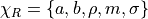$\chi_R = \{a, b, \rho, m, \sigma \}$ is the SVI parameter set where:

$a$ controls the level of the variance
$b$ controls the wings of both the put and call wings
Increasing $\rho$ decreases(increases) the slope of the left(right) wing
Increasing $m$ translates the smile to the right
Increasing $\sigma$ reduces the at the money (ATM) curvature of the smile

class ql.SviSmileSection(timeToExpiry: float, forward: float, sviParameters: List[float])

Constructs an SVI smile section using an expiry time (in year fractions).

Parameters:

timeToExpiry (float) – The time to expiry in year fractions.
forward (float) – The forward rate or spot price at expiry.
sviParameters (List[float]) –
A list of SVI model parameters [a, b, sigma, rho, m]:
- a (float): The minimum variance level. Controls the overall volatility floor.
- b (float): The smile amplitude parameter. Controls the overall curvature and depth of the smile.
- m (float): The smile location (moneyness shift). Controls the skew position.
- rho (float): The skew parameter in the range [-1, 1]. Controls the direction and asymmetry of the smile.
- sigma (float): The volatility of volatility parameter. Controls the convexity of the smile.

class ql.SviSmileSection(date: ql.Date, forward: float, sviParameters: List[float], dc: ql.DayCounter = ql.Actual365Fixed())

Constructs an SVI smile section using an expiry date.

Parameters:

date (ql.Date) – The expiry date for this smile section.
forward (float) – The forward rate or spot price at the expiry date.
sviParameters (List[float]) – A list of SVI model parameters [a, b, sigma, rho, m] (see constructor above for details).
dc (ql.DayCounter) – The day-count convention used to compute the time to expiry (default is Actual365Fixed).

Example usage:

# SVI parameters
 a = -0.0666
 b = 0.229
 m = 0.193
 rho = 0.439
 sigma = 0.337

 # Using expiry time (in years)
 time_to_expiry = 0.25  # 3 months
 forward_rate = 100

 smile = ql.SviSmileSection(time_to_expiry, forward_rate, [a, b, sigma, rho, m])

 # Using expiry date
 expiry_date = ql.Date(15, 3, 2026)  # 15 March 2026
 dayCounter = ql.Actual365Fixed()

 smile_by_date = ql.SviSmileSection(expiry_date, forward_rate, [a, b, sigma, rho, m], dayCounter)

 # Query volatility at different strikes
 atm_vol = smile.volatility(forward_rate)
 otm_call_vol = smile.volatility(forward_rate * 1.10)
 otm_put_vol = smile.volatility(forward_rate * 0.90)

SviInterpolatedSmileSection

An interpolated smile section that uses the SVI (Stochastic Volatility Inspired) model to fit and calibrate the volatility smile from a set of market option quotes. Unlike the parametric ql.SviSmileSection, this class calibrates the SVI parameters to match observed market volatilities at specific strikes, making it more flexible for real-world market data fitting.

The SVI model is calibrated by minimizing the difference between the model-implied volatilities and the market-observed volatilities at the given strikes.

class ql.SviInterpolatedSmileSection(optionDate: ql.Date, forward: QuoteHandle, strikes: List[float], hasFloatingStrikes: bool, atmVolatility: QuoteHandle, volHandles: List[QuoteHandle], a: float, b: float, sigma: float, rho: float, m: float, aIsFixed: bool, bIsFixed: bool, sigmaIsFixed: bool, rhoIsFixed: bool, mIsFixed: bool, vegaWeighted: bool = True, endCriteria: ql.EndCriteria = None, method: ql.OptimizationMethod = None, dc: ql.DayCounter = ql.Actual365Fixed())

Constructs an SVI interpolated smile section using floating market data (Quotes).

This constructor is useful when market data is dynamic and needs to be updated in real-time.

Parameters:

optionDate (ql.Date) – The expiry date for this smile section.
forward (ql.QuoteHandle) – Handle to a quote representing the forward rate or spot price at expiry.
strikes (List[float]) – A list of strike rates at which market volatilities are observed.
hasFloatingStrikes (bool) – Boolean flag indicating whether strikes are floating (Quote handles) or fixed. Set to True for floating strikes, False for fixed.
atmVolatility (ql.QuoteHandle) – Handle to a quote representing the at-the-money (ATM) volatility.
volHandles (List[ql.QuoteHandle]) – A list of QuoteHandle objects representing the market volatilities at each corresponding strike.
a (float) – Initial guess for the SVI parameter a (minimum variance level).
b (float) – Initial guess for the SVI parameter b (smile amplitude).
sigma (float) – Initial guess for the SVI parameter sigma (volatility of volatility).
rho (float) – Initial guess for the SVI parameter rho (skew/correlation parameter, typically in [-1, 1]).
m (float) – Initial guess for the SVI parameter m (smile location/moneyness shift).
aIsFixed (bool) – If True, the parameter a is held fixed during calibration; if False, it is optimized.
bIsFixed (bool) – If True, the parameter b is held fixed; if False, it is optimized.
sigmaIsFixed (bool) – If True, the parameter sigma is held fixed; if False, it is optimized.
rhoIsFixed (bool) – If True, the parameter rho is held fixed; if False, it is optimized.
mIsFixed (bool) – If True, the parameter m is held fixed; if False, it is optimized.
vegaWeighted (bool) – If True, the calibration uses vega-weighted least squares, giving more weight to options near the ATM. Default is True.
endCriteria (ql.EndCriteria or None) – Optional ql.EndCriteria object specifying stopping conditions for the optimization (e.g., tolerance, max iterations). If None, default criteria are used.
method (ql.OptimizationMethod or None) – Optional ql.OptimizationMethod object specifying the numerical optimization algorithm (e.g., Levenberg-Marquardt, Simplex). If None, a default method is used.
dc (ql.DayCounter) – Day-count convention used to compute the time to expiry. Default is Actual365Fixed.

class ql.SviInterpolatedSmileSection(optionDate: ql.Date, forward: float, strikes: List[float], hasFloatingStrikes: bool, atmVolatility: float, vols: List[float], a: float, b: float, sigma: float, rho: float, m: float, aIsFixed: bool, bIsFixed: bool, sigmaIsFixed: bool, rhoIsFixed: bool, mIsFixed: bool, vegaWeighted: bool = True, endCriteria: ql.EndCriteria = None, method: ql.OptimizationMethod = None, dc: ql.DayCounter = ql.Actual365Fixed())

Constructs an SVI interpolated smile section using fixed market data (scalar values).

This constructor is useful when working with static market snapshots or historical data.

Parameters:

optionDate (ql.Date) – The expiry date for this smile section.
forward (float) – The forward rate or spot price at expiry.
strikes (List[float]) – A list of strike rates at which market volatilities are observed.
hasFloatingStrikes (bool) – Boolean flag indicating whether strikes are floating or fixed. Set to False when strikes are fixed scalars.
atmVolatility (float) – The at-the-money (ATM) volatility value.
vols (List[float]) – A list of market volatilities corresponding to each strike.
a (float) – Initial guess for the SVI parameter a (minimum variance level).
b (float) – Initial guess for the SVI parameter b (smile amplitude).
sigma (float) – Initial guess for the SVI parameter sigma (volatility of volatility).
rho (float) – Initial guess for the SVI parameter rho (skew/correlation parameter).
m (float) – Initial guess for the SVI parameter m (smile location).
aIsFixed (bool) – If True, parameter a is fixed; if False, it is optimized.
bIsFixed (bool) – If True, parameter b is fixed; if False, it is optimized.
sigmaIsFixed (bool) – If True, parameter sigma is fixed; if False, it is optimized.
rhoIsFixed (bool) – If True, parameter rho is fixed; if False, it is optimized.
mIsFixed (bool) – If True, parameter m is fixed; if False, it is optimized.
vegaWeighted (bool) – If True, uses vega-weighted least squares. Default is True.
endCriteria (ql.EndCriteria or None) – Optional optimization end criteria. Default is None.
method (ql.OptimizationMethod or None) – Optional optimization method. Default is None.
dc (ql.DayCounter) – Day-count convention. Default is Actual365Fixed.

Methods

a()

Returns the calibrated SVI parameter a (minimum variance level).

Returns:: The a parameter value.
Return type:: float

b()

Returns the calibrated SVI parameter b (smile amplitude).

Returns:: The b parameter value.
Return type:: float

sigma()

Returns the calibrated SVI parameter sigma (volatility of volatility).

Returns:: The sigma parameter value.
Return type:: float

rho()

Returns the calibrated SVI parameter rho (skew/correlation).

Returns:: The rho parameter value.
Return type:: float

m()

Returns the calibrated SVI parameter m (smile location).

Returns:: The m parameter value.
Return type:: float

rmsError()

Returns the root-mean-square (RMS) error of the fit, indicating the average deviation between model and market volatilities.

Returns:: The RMS error of the calibration.
Return type:: float

maxError()

Returns the maximum absolute error across all strikes, indicating the worst-fit point.

Returns:: The maximum error of the calibration.
Return type:: float

endCriteria()

Returns the end criteria type that was met during the optimization (e.g., convergence, max iterations reached).

Returns:: The end criteria type.
Return type:: ql.EndCriteria.Type

Example usage:

today = ql.Date(15, 12, 2025)
ql.Settings.instance().evaluationDate = today
expiry_date = ql.Date(15, 3, 2026)  # 3 months
dayCounter = ql.Actual365Fixed()

# Market data
forward = 100.0
atm_vol = 0.20
strikes = [90.0, 95.0, 100.0, 105.0, 110.0]
market_vols = [0.25, 0.22, 0.20, 0.22, 0.25]  # Volatility smile

# SVI initial parameter guesses
a_init = 0.05
b_init = 0.3
sigma_init = 0.5
rho_init = -0.2
m_init = 0.0

# Calibrate SVI smile section (optimize all parameters)
smile = ql.SviInterpolatedSmileSection(
    expiry_date,
    forward,
    strikes,
    False,  # hasFloatingStrikes = False (fixed market data)
    atm_vol,
    market_vols,
    a_init, b_init, sigma_init, rho_init, m_init,
    False, False, False, False, False,  # All parameters free to optimize
    True # Vega weighted
)

# Access calibrated parameters
print(f"Calibrated a: {smile.a()}")
print(f"Calibrated b: {smile.b()}")
print(f"Calibrated sigma: {smile.sigma()}")
print(f"Calibrated rho: {smile.rho()}")
print(f"Calibrated m: {smile.m()}")
print(f"RMS Error: {smile.rmsError()}")
print(f"Max Error: {smile.maxError()}")

# Query implied volatility at any strike
implied_vol_105 = smile.volatility(105.0)
print(f"Implied vol at 105: {implied_vol_105}")

# Example with some parameters fixed
smile_partial = ql.SviInterpolatedSmileSection(
    expiry_date,
    forward,
    strikes,
    False,
    atm_vol,
    market_vols,
    a_init, b_init, sigma_init, rho_init, m_init,
    True,   # Fix a
    False,  # Optimize b
    False,  # Optimize sigma
    False,  # Optimize rho
    True,   # Fix m
    True # Vega weighted
)

Note

Calibration Tips:

Start with reasonable initial guesses for SVI parameters to aid convergence.
Use vegaWeighted=True to give more importance to near-the-money options, which are typically more liquid.
Check rmsError() and maxError() to assess fit quality.
Fix parameters (e.g., mIsFixed=True) if you have external constraints or want to stabilize the calibration.
For custom optimization, pass custom ql.EndCriteria and ql.OptimizationMethod objects.

KahaleSmileSection

A smile section that applies the Kahale arbitrage-removal algorithm to an existing ql.SmileSection. The Kahale method is a sophisticated technique that removes calendar and butterfly arbitrage from volatility smiles while preserving the original smile shape as much as possible. It’s particularly useful for regularizing market-implied volatility smiles that may contain arbitrage opportunities due to market frictions or data quality issues.

The algorithm constructs a C1-continuous (smooth, differentiable) curve that is arbitrage-free and stays as close as possible to the input smile section.

class ql.KahaleSmileSection(source: ql.SmileSection, atm: float = None, interpolate: bool = False, exponentialExtrapolation: bool = False, deleteArbitragePoints: bool = False, moneynessGrid: list[float] = None, gap: float = 1.0e-5, forcedLeftIndex: int = -1, forcedRightIndex: int = 2147483647)

Constructs a Kahale-regularized smile section from an input smile section.

Parameters:

source (ql.SmileSection) – The input smile section to be regularized. Must be a valid ql.SmileSection object.
atm (float or None) – Optional override for the at-the-money (ATM) level. If not provided (None), the ATM level from the source smile section is used. This is useful when you want to shift the reference point for moneyness.
interpolate (bool) – If True, the algorithm will interpolate the smile between the discrete moneyness grid points. If False (default), only the grid points are used. Set to True for smoother extrapolation behavior.
exponentialExtrapolation (bool) – If True, the smile is extrapolated using an exponential model for strikes far from the ATM. If False (default), a linear or flatter extrapolation is used. Exponential extrapolation is more realistic for extreme moneyness but can be less stable.
deleteArbitragePoints (bool) – If True, the algorithm will remove (skip) grid points that contain arbitrage violations. This can reduce the number of calibration points. If False (default), all points are preserved and adjusted.
moneynessGrid (list[float] or None) – Optional custom list of moneyness points (strike / ATM) at which the smile is evaluated. If not provided (empty or None), a default grid is constructed from the source smile section. Providing a custom grid allows fine-tuning the regularization.
gap (float) – Finite-difference gap size (in absolute terms, not moneyness) used to compute numerical derivatives when checking for arbitrage. Smaller gaps give more precise arbitrage detection but can be numerically sensitive. Default is 1.0e-5.
forcedLeftIndex (int) – Index of a specific point to be forced as a left boundary in the regularization. Set to -1 (default) to auto-select. Use this to pin the left wing of the smile at a specific moneyness point.
forcedRightIndex (int) – Index of a specific point to be forced as a right boundary in the regularization. Set to 2147483647 (default QL_MAX_INTEGER) to auto-select. Use this to pin the right wing of the smile at a specific moneyness point.

Example usage — Basic arbitrage removal:

import QuantLib as ql
import numpy as np

# Setup
today = ql.Date(15, 12, 2025)
ql.Settings.instance().evaluationDate = today
expiry_date = ql.Date(15, 3, 2026)  # 3 months
dayCounter = ql.Actual365Fixed()

# Create an input smile section with potential arbitrage
# (e.g., from market data or interpolation)
forward = 100.0
atm_vol = 0.20
strikes = [80.0, 90.0, 100.0, 110.0, 120.0]
market_vols = [0.30, 0.22, 0.20, 0.22, 0.30]

# Build the input smile using spline interpolation
smile_input = ql.SplineCubicInterpolatedSmileSection(
    expiry_date,
    strikes,
    [v * np.sqrt(0.25) for v in market_vols],  # Convert to std-dev
    100.0,
    dayCounter
)

# Apply Kahale regularization to remove arbitrage
smile_kahale = ql.KahaleSmileSection(
    smile_input,
    forward,
    True,
    False,
    False
)

# Query volatility from the arbitrage-free smile
vol_atm = smile_kahale.volatility(forward)
vol_otm_call = smile_kahale.volatility(110.0)
vol_otm_put = smile_kahale.volatility(90.0)

print(f"ATM vol (regularized): {vol_atm:.4f}")
print(f"OTM call vol: {vol_otm_call:.4f}")
print(f"OTM put vol: {vol_otm_put:.4f}")

Example usage — Custom moneyness grid with exponential extrapolation:

# Custom moneyness grid (fine-grained near ATM, coarser in wings)
custom_moneyness = [0.70, 0.80, 0.90, 0.95, 1.00, 1.05, 1.10, 1.20, 1.30]

# Apply Kahale with custom grid and exponential extrapolation
smile_kahale_custom = ql.KahaleSmileSection(
    smile_input,
    forward,
    True,
    True,  # Use exponential tails
    False,
    ustom_moneyness
)

# Evaluate smile at various strikes
test_strikes = [70.0, 80.0, 90.0, 100.0, 110.0, 120.0, 130.0]
for strike in test_strikes:
    vol = smile_kahale_custom.volatility(strike)
    print(f"Strike {strike}: vol = {vol:.4f}")

Example usage — Aggressive arbitrage removal with point deletion:

# More aggressive: remove points that violate arbitrage constraints
smile_kahale_aggressive = ql.KahaleSmileSection(
    smile_input,
    forward,
    True,
    True,
    True,  # Remove problematic points
    [],
    1.0e-4  # Slightly larger finite-difference step
)

print(f"Regularized ATM vol: {smile_kahale_aggressive.volatility(forward):.4f}")

Note

When to use KahaleSmileSection:

Market-implied smiles may contain micro-structure noise or arbitrage due to bid-ask spreads.
Interpolated smiles (e.g., cubic spline) can exhibit arbitrage between input points.
Risk management: Arbitrage-free surfaces are essential for consistent pricing across strikes.
Model calibration: Use before calibrating stochastic volatility models to ensure consistency.

Warning

The Kahale algorithm is computationally intensive; use only when arbitrage-free properties are critical.
The regularized smile may deviate noticeably from the input smile if the input contains substantial arbitrage.
For very sparse or low-quality input data, consider increasing gap or enabling deleteArbitragePoints for more stable results.

EquityFX

BlackVolTermStructure

The base abstract class of all the EquityFX volatility termstructures is the BlackVolTermStructure which represents the Black (lognormal) volatility surface as a function of expiry date and strike. This class defines the core interface for querying volatilities and variances at arbitrary combinations of dates and strikes, with support for both spot and forward volatility queries.

The BlackVolTermStructure is an abstract class and cannot be instantiated directly. Instead, use concrete implementations such as ql.BlackConstantVol, ql.BlackVarianceCurve, or ql.BlackVarianceSurface.

Methods

blackVol(expiryDate: ql.Date, strike: float, extrapolate: bool = False)

Returns the Black (lognormal) implied volatility at a given expiry date and strike.

This method queries the volatility surface at the specified date and strike level. The result can be used for option pricing, greeks computation, and risk management.

Parameters:

expiryDate (ql.Date) – The expiry (exercise) date for which volatility is requested.
strike (float) – The strike price at which volatility is requested.
extrapolate (bool) – If False (default), an exception is raised if the query point (date, strike) is outside the range of the available data. If True, the surface is extrapolated beyond its boundaries using the interpolator’s default extrapolation method.

Returns:

The Black volatility (annualized, as a decimal) at the given expiry and strike.

Return type:

float

Raises:

Raises an exception if the query point is out of range and extrapolate=False.

blackVol(expiryTime: float, strike: float, extrapolate: bool = False)

Returns the Black (lognormal) implied volatility at a given expiry time (in year fractions) and strike.

This is an alternative method signature that takes time (instead of a date) as input, useful when working with time-based calculations.

Parameters:

expiryTime (float) – The time to expiry in year fractions (computed using the day-count convention).
strike (float) – The strike price.
extrapolate (bool) – Whether to extrapolate beyond the data range (default is False).

Returns:

The Black volatility at the given expiry time and strike.

Return type:

float

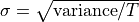
blackVariance(expiryDate: ql.Date, strike: float, extrapolate: bool = False)

Returns the total variance (volatility squared times time) at a given expiry date and strike.

Total variance is equal to $\sigma^2 \times T$ , where $\sigma$ is the volatility and $T$ is the time to expiry. This quantity is useful for option pricing formulas and volatility interpolation.

Parameters:

expiryDate (ql.Date) – The expiry date for which variance is requested.
strike (float) – The strike price.
extrapolate (bool) – Whether to extrapolate beyond the data range (default is False).

Returns:

The total variance at the given expiry date and strike.

Return type:

float

Note

Total variance = (Black volatility)² × (time to expiry). To recover volatility, take $\sigma = \sqrt{\text{variance} / T}$ .

blackVariance(expiryTime: float, strike: float, extrapolate: bool = False)

Returns the total variance at a given expiry time (in year fractions) and strike.

This is an alternative method signature that takes time instead of a date.

Parameters:

expiryTime (float) – The time to expiry in year fractions.
strike (float) – The strike price.
extrapolate (bool) – Whether to extrapolate beyond the data range.

Returns:

The total variance.

Return type:

float

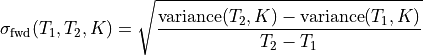
blackForwardVol(expiryDate1: ql.Date, expiryDate2: ql.Date, strike: float, extrapolate: bool = False)

Returns the forward volatility between two dates at a given strike.

Forward volatility is the volatility applicable to the period between expiryDate1 and expiryDate2, computed from the spot volatility surface. This is useful for pricing forward-starting options and understanding future volatility expectations.

Forward volatility is computed from the spot variances using:

$\sigma_{\text{fwd}}(T_1, T_2, K) = \sqrt{\frac{\text{variance}(T_2, K) - \text{variance}(T_1, K)}{T_2 - T_1}}$

Parameters:

expiryDate1 (ql.Date) – The start date of the forward period. Must be before or equal to expiryDate2.
expiryDate2 (ql.Date) – The end date of the forward period.
strike (float) – The strike price.
extrapolate (bool) – Whether to extrapolate beyond the data range (default is False).

Returns:

The forward volatility between the two dates at the given strike.

Return type:

float

Raises:

Raises an exception if expiryDate1 > expiryDate2.

blackForwardVol(expiryTime1: float, expiryTime2: float, strike: float, extrapolate: bool = False)

Returns the forward volatility between two times (in year fractions) at a given strike.

This is an alternative method signature that takes time instead of dates.

Parameters:

expiryTime1 (float) – The start time in year fractions. Must be less than or equal to expiryTime2.
expiryTime2 (float) – The end time in year fractions.
strike (float) – The strike price.
extrapolate (bool) – Whether to extrapolate beyond the data range.

Returns:

The forward volatility.

Return type:

float

blackForwardVariance(expiryDate1: ql.Date, expiryDate2: ql.Date, strike: float, extrapolate: bool = False)

Returns the forward variance between two dates at a given strike.

Forward variance is related to forward volatility by: forward variance = (forward volatility)² × (time difference). This quantity is useful for option pricing and variance-based calculations.

Forward variance is computed from spot variances as:

$\text{variance}_{\text{fwd}}(T_1, T_2, K) = \text{variance}(T_2, K) - \text{variance}(T_1, K)$

Parameters:

expiryDate1 (ql.Date) – The start date of the forward period.
expiryDate2 (ql.Date) – The end date of the forward period.
strike (float) – The strike price.
extrapolate (bool) – Whether to extrapolate beyond the data range.

Returns:

The forward variance between the two dates.

Return type:

float

blackForwardVariance(expiryTime1: float, expiryTime2: float, strike: float, extrapolate: bool = False)

Returns the forward variance between two times (in year fractions) at a given strike.

This is an alternative method signature that takes time instead of dates.

Parameters:

expiryTime1 (float) – The start time in year fractions.
expiryTime2 (float) – The end time in year fractions.
strike (float) – The strike price.
extrapolate (bool) – Whether to extrapolate beyond the data range.

Returns:

The forward variance.

Return type:

float

BlackConstantVol

A constant Black (lognormal) volatility structure $\sigma: (k, t) \rightarrow \sigma \in \mathbb{R}$ . This is the simplest volatility model where the volatility is flat across all expiry dates, strikes, and the evaluation date. It is commonly used as a baseline model for option pricing and risk management when more sophisticated volatility surfaces are not available or necessary.

class ql.BlackConstantVol(referenceDate: ql.Date, calendar: ql.Calendar, volatility: float, dayCounter: ql.DayCounter)

Constructs a constant Black volatility structure using a fixed reference date and a scalar volatility value.

Parameters:

referenceDate (ql.Date) – The reference (valuation) date for the volatility structure. All forward dates are measured relative to this date.
calendar (ql.Calendar) – The calendar used for date calculations and business day conventions.
volatility (float) – The constant Black (lognormal) volatility value (annualized, expressed as a decimal). For example, 0.20 represents 20% volatility.
dayCounter (ql.DayCounter) – The day-count convention used to convert dates to year fractions (time to expiry).

class ql.BlackConstantVol(referenceDate: ql.Date, calendar: ql.Calendar, volatility: ql.QuoteHandle, dayCounter: ql.DayCounter)

Constructs a constant Black volatility structure using a fixed reference date and a floating volatility quote.

This constructor allows the volatility to be updated dynamically through the underlying quote.

Parameters:

referenceDate (ql.Date) – The reference (valuation) date for the volatility structure.
calendar (ql.Calendar) – The calendar used for date calculations.
volatility (ql.QuoteHandle) – A handle to a quote representing the constant Black volatility. Changes to the underlying quote are immediately reflected in the volatility structure.
dayCounter (ql.DayCounter) – The day-count convention used to compute year fractions.

class ql.BlackConstantVol(settlementDays: int, calendar: ql.Calendar, volatility: float, dayCounter: ql.DayCounter)

Constructs a constant Black volatility structure using a floating reference date (settlement days) and a scalar volatility value.

The reference date is computed as the settlement date (today + settlementDays) and updates dynamically as the evaluation date changes.

Parameters:

settlementDays (int) – The number of business days used to compute the reference date from the evaluation date. The reference date is automatically updated when the evaluation date changes.
calendar (ql.Calendar) – The calendar used for date calculations and business day conventions.
volatility (float) – The constant Black (lognormal) volatility value (annualized, as a decimal).
dayCounter (ql.DayCounter) – The day-count convention used to convert dates to year fractions.

class ql.BlackConstantVol(settlementDays: int, calendar: ql.Calendar, volatility: ql.QuoteHandle, dayCounter: ql.DayCounter)

Constructs a constant Black volatility structure using a floating reference date (settlement days) and a floating volatility quote.

Both the reference date and volatility are dynamic and update as the evaluation date and quote values change.

Parameters:

settlementDays (int) – The number of business days used to compute the reference date.
calendar (ql.Calendar) – The calendar used for date calculations.
volatility (ql.QuoteHandle) – A handle to a quote representing the constant Black volatility.
dayCounter (ql.DayCounter) – The day-count convention used to compute year fractions.

Example usage — Fixed reference date with constant volatility:

import QuantLib as ql

referenceDate = ql.Date(15, 12, 2025)
calendar = ql.TARGET()
volatility = 0.20  # 20% constant volatility
dayCounter = ql.Actual360()

# Create constant volatility structure with fixed reference date
constVol = ql.BlackConstantVol(referenceDate, calendar, volatility, dayCounter)

# Query volatility at any date and strike
expiryDate = ql.Date(15, 3, 2026)  # 3 months
strike = 100.0

vol = constVol.blackVol(expiryDate, strike)
print(f"Black vol at strike {strike}: {vol:.4f}")  # Output: 0.2000

Example usage — Floating reference date (settlement days) with constant volatility:

settlementDays = 2
calendar = ql.TARGET()
volatility = 0.25  # 25% constant volatility
dayCounter = ql.Actual365Fixed()

# Create constant volatility structure with floating reference date
constVol_floating = ql.BlackConstantVol(settlementDays, calendar, volatility, dayCounter)

# The reference date is automatically computed from the evaluation date
today = ql.Date(15, 12, 2025)
ql.Settings.instance().evaluationDate = today

expiryDate = ql.Date(15, 6, 2026)  # 6 months
vol = constVol_floating.blackVol(expiryDate, 105.0)
print(f"Black vol: {vol:.4f}")  # Output: 0.2500

# Update the evaluation date; reference date automatically updates
tomorrow = ql.Date(16, 12, 2025)
ql.Settings.instance().evaluationDate = tomorrow

vol_next = constVol_floating.blackVol(expiryDate, 105.0)
print(f"Black vol after date change: {vol_next:.4f}")

Example usage — Fixed reference date with dynamic volatility (QuoteHandle):

referenceDate = ql.Date(15, 12, 2025)
calendar = ql.TARGET()
dayCounter = ql.Actual360()

# Create a volatility quote that can be updated
volQuote = ql.SimpleQuote(0.20)
volHandle = ql.QuoteHandle(volQuote)

# Create constant volatility structure with dynamic volatility
constVol_dynamic = ql.BlackConstantVol(referenceDate, calendar, volHandle, dayCounter)

expiryDate = ql.Date(15, 3, 2026)
strike = 100.0

# Query initial volatility
vol_initial = constVol_dynamic.blackVol(expiryDate, strike)
print(f"Initial Black vol: {vol_initial:.4f}")  # Output: 0.2000

# Update the volatility quote
volQuote.setValue(0.25)

# Query updated volatility
vol_updated = constVol_dynamic.blackVol(expiryDate, strike)
print(f"Updated Black vol: {vol_updated:.4f}")  # Output: 0.2500

Example usage — Floating reference date with dynamic volatility:

settlementDays = 2
calendar = ql.TARGET()
dayCounter = ql.Actual365Fixed()

# Create a volatility quote
volQuote = ql.SimpleQuote(0.18)
volHandle = ql.QuoteHandle(volQuote)

# Create constant volatility structure with both floating reference date and dynamic volatility
constVol_full_dynamic = ql.BlackConstantVol(settlementDays, calendar, volHandle, dayCounter)

today = ql.Date(15, 12, 2025)
ql.Settings.instance().evaluationDate = today

expiryDate = ql.Date(15, 9, 2026)  # 9 months

vol = constVol_full_dynamic.blackVol(expiryDate, 100.0)
print(f"Black vol: {vol:.4f}")  # Output: 0.1800

# Update both the evaluation date and volatility
ql.Settings.instance().evaluationDate = ql.Date(16, 12, 2025)
volQuote.setValue(0.22)

vol_updated = constVol_full_dynamic.blackVol(expiryDate, 100.0)
print(f"Updated Black vol: {vol_updated:.4f}")  # Output: 0.2200

BlackVarianceCurve

A volatility curve $\sigma: t \rightarrow \sigma(t) \in \mathbb{R}$ representing the Black (lognormal) volatility as a function of expiry date only. This curve provides volatility values at arbitrary expiry dates within the range of the input data through interpolation.

The curve uses a term structure of Black variances (not volatilities directly) to ensure consistency and smooth interpolation. By default, the curve enforces monotone variance (which means that variance must be non-decreasing), which prevents calendar arbitrage opportunities in the volatility term structure.

class ql.BlackVarianceCurve(referenceDate: ql.Date, dates: List[ql.Date], volatilities: List[float], dayCounter: ql.DayCounter, forceMonotoneVariance: bool = True)

Constructs a Black variance curve from a vector of expiry dates and their corresponding volatilities.

Parameters:

referenceDate (ql.Date) – The reference (valuation) date for the curve. All expiry dates are measured relative to this date.
dates (List[ql.Date]) – A list of expiry dates corresponding to the input volatility values. Dates must be in strictly increasing order.
volatilities (List[float]) – A list of Black (lognormal) volatilities corresponding to each expiry date. These are annualized implied volatilities (not variances).
dayCounter (ql.DayCounter) – The day-count convention used to convert dates to year fractions (time to expiry).
forceMonotoneVariance (bool) – If True (default), the curve enforces monotone increasing variance, which prevents calendar arbitrage. If False, the raw interpolation of the input volatilities is used without variance monotonicity constraints. Default is True.

Example usage — Basic construction with monotone variance enforcement:

import QuantLib as ql

# Setup
referenceDate = ql.Date(30, 9, 2013)
ql.Settings.instance().evaluationDate = referenceDate
dayCounter = ql.Actual360()

# Expiry dates and corresponding volatilities
expirations = [
    ql.Date(20, 12, 2013),  # ~2.8 months
    ql.Date(17, 1, 2014),   # ~3.6 months
    ql.Date(21, 3, 2014)    # ~6 months
]
volatilities = [0.145, 0.156, 0.165]

# Create volatility curve (enforces monotone variance by default)
volatilityCurve = ql.BlackVarianceCurve(
    referenceDate,
    expirations,
    volatilities,
    dayCounter
)
volatilityCurve.enableExtrapolation()

# Query volatility at specific expiry dates
vol_at_first = volatilityCurve.blackVol(expirations[0])
vol_at_second = volatilityCurve.blackVol(expirations[1])

print(f"Vol at {expirations[0]}: {vol_at_first:.4f}")
print(f"Vol at {expirations[1]}: {vol_at_second:.4f}")

# Query volatility at intermediate dates (via interpolation)
intermediate_date = ql.Date(10, 1, 2014)  # Between first and second expiry
vol_intermediate = volatilityCurve.blackVol(intermediate_date)
print(f"Interpolated vol at {intermediate_date}: {vol_intermediate:.4f}")

BlackVarianceSurface

A volatility surface $\sigma: (k, t) \rightarrow \sigma(k, t) \in \mathbb{R}$ representing the Black (lognormal) volatility as a function of both expiry date and strike. This surface uses 2D interpolation to provide volatility values at arbitrary combinations of expiry and strike that are within the range of the input data.

The surface supports two interpolation methods (Bilinear and Bicubic) and allows customization of how the surface behaves beyond the bounds of the input data (extrapolation behavior).

class ql.BlackVarianceSurface(referenceDate: ql.Date, calendar: ql.Calendar, expirations: List[ql.Date], strikes: List[float], volMatrix: ql.Matrix, dayCounter: ql.DayCounter, lowerExtrapolation: ql.BlackVarianceSurface.Extrapolation = ql.BlackVarianceSurface.InterpolatorDefaultExtrapolation, upperExtrapolation: ql.BlackVarianceSurface.Extrapolation = ql.BlackVarianceSurface.InterpolatorDefaultExtrapolation, interpolator: str = 'bilinear')

Constructs a Black variance surface from a matrix of volatilities.

Parameters:

referenceDate (ql.Date) – The reference (valuation) date for the surface.
calendar (ql.Calendar) – The calendar used for date calculations and settlement conventions.
expirations (List[ql.Date]) – A list of expiry dates corresponding to the columns of the volatility matrix.
strikes (List[float]) – A list of strike prices corresponding to the rows of the volatility matrix.
volMatrix (ql.Matrix) – A matrix of Black (lognormal) volatilities where rows correspond to strikes and columns correspond to expirations. Dimensions must be len(strikes) x len(expirations).
dayCounter (ql.DayCounter) – The day-count convention used to compute time to expiry (year fractions).
lowerExtrapolation (ql.BlackVarianceSurface.Extrapolation) – Extrapolation strategy for strikes below the minimum strike in the input data. Can be ql.BlackVarianceSurface.ConstantExtrapolation (flat volatility) or ql.BlackVarianceSurface.InterpolatorDefaultExtrapolation (uses interpolator’s default behavior). Default is InterpolatorDefaultExtrapolation.
upperExtrapolation (ql.BlackVarianceSurface.Extrapolation) – Extrapolation strategy for strikes above the maximum strike in the input data. Can be ql.BlackVarianceSurface.ConstantExtrapolation (flat volatility) or ql.BlackVarianceSurface.InterpolatorDefaultExtrapolation (uses interpolator’s default behavior). Default is InterpolatorDefaultExtrapolation.
interpolator (str) – The interpolation method to use for the 2D surface. Supported values are "bilinear" (default) or "bicubic". The default is used if an empty string is provided.

Methods

setInterpolation(interpolator: str = 'bilinear')

Sets or changes the interpolation method used for the volatility surface.

Parameters:: interpolator (str) – The interpolation method to use. Supported values are "bilinear" or "bicubic". If an empty string is provided, defaults to "bilinear". Case-insensitive.
Raises:: Raises an exception if the interpolator name is not recognized.

Extrapolation Enum

The BlackVarianceSurface.Extrapolation enumeration defines how the surface behaves for strikes outside the range of the input data:

ql.BlackVarianceSurface.ConstantExtrapolation: The volatility at the boundary (minimum or maximum strike) is used as a flat constant for all strikes beyond that boundary.
ql.BlackVarianceSurface.InterpolatorDefaultExtrapolation: Uses the default extrapolation behavior of the chosen interpolator (bilinear or bicubic). This typically results in linear extrapolation in the strike dimension.

Example usage — Basic construction with default bilinear interpolation:

referenceDate = ql.Date(30, 9, 2013)
ql.Settings.instance().evaluationDate = referenceDate
calendar = ql.TARGET()
dayCounter = ql.ActualActual()

strikes = [1650.0, 1660.0, 1670.0]
expirations = [ql.Date(20, 12, 2013), ql.Date(17, 1, 2014), ql.Date(21, 3, 2014)]

volMatrix = ql.Matrix(len(strikes), len(expirations))

# 1650 - Dec, Jan, Mar
volMatrix[0][0] = 0.15640; volMatrix[0][1] = 0.15433; volMatrix[0][2] = 0.16079
# 1660 - Dec, Jan, Mar
volMatrix[1][0] = 0.15343; volMatrix[1][1] = 0.15240; volMatrix[1][2] = 0.15804
# 1670 - Dec, Jan, Mar
volMatrix[2][0] = 0.15128; volMatrix[2][1] = 0.14888; volMatrix[2][2] = 0.15512

# Create surface with default bilinear interpolation
volatilitySurface = ql.BlackVarianceSurface(
    referenceDate,
    calendar,
    expirations,
    strikes,
    volMatrix,
    dayCounter
)
volatilitySurface.enableExtrapolation()

# Query volatility at specific strike and expiry
strike = 1665.0
expiry = ql.Date(20, 12, 2013)
vol = volatilitySurface.blackVol(expiry, strike)
print(f"Volatility at strike {strike}, expiry {expiry}: {vol:.4f}")

Example usage — Construction with explicit bicubic interpolation:

# Create surface with bicubic interpolation for smoother surface
volatilitySurface_bicubic = ql.BlackVarianceSurface(
    referenceDate,
    calendar,
    expirations,
    strikes,
    volMatrix,
    dayCounter,
    ql.BlackVarianceSurface.ConstantExtrapolation,
    ql.BlackVarianceSurface.ConstantExtrapolation,
    "bicubic"  # Use bicubic instead of bilinear
)
volatilitySurface_bicubic.enableExtrapolation()

vol_bicubic = volatilitySurface_bicubic.blackVol(ql.Date(20, 12, 2013), 1665.0)
print(f"Bicubic interpolated vol: {vol_bicubic:.4f}")

Example usage — Switching interpolation methods:

# Start with bilinear interpolation
volatilitySurface = ql.BlackVarianceSurface(
    referenceDate,
    calendar,
    expirations,
    strikes,
    volMatrix,
    dayCounter
)

# Switch to bicubic interpolation
volatilitySurface.setInterpolation("bicubic")
vol_after_switch = volatilitySurface.blackVol(ql.Date(20, 12, 2013), 1660.0)
print(f"Volatility with bicubic: {vol_after_switch:.4f}")

# Switch back to bilinear (or use empty string for default)
volatilitySurface.setInterpolation("")  # Defaults to bilinear
vol_bilinear = volatilitySurface.blackVol(ql.Date(20, 12, 2013), 1660.0)
print(f"Volatility with bilinear: {vol_bilinear:.4f}")

HestonBlackVolSurface

class ql.HestonBlackVolSurface(hestonModelHandle)

flatTs = ql.YieldTermStructureHandle(
  ql.FlatForward(ql.Date().todaysDate(), 0.05, ql.Actual365Fixed())
)
dividendTs = ql.YieldTermStructureHandle(
  ql.FlatForward(ql.Date().todaysDate(), 0.02, ql.Actual365Fixed())
)

v0 = 0.01; kappa = 0.01; theta = 0.01; rho = 0.0; sigma = 0.01
spot = 100
process = ql.HestonProcess(flatTs, dividendTs,
                            ql.QuoteHandle(ql.SimpleQuote(spot)),
                            v0, kappa, theta, sigma, rho
                            )

hestonModel = ql.HestonModel(process)
hestonHandle = ql.HestonModelHandle(hestonModel)
hestonVolSurface = ql.HestonBlackVolSurface(hestonHandle)

AndreasenHugeVolatilityAdapter

An implementation of the arb-free Andreasen-Huge vol interpolation described in “Andreasen J., Huge B., 2010. Volatility Interpolation” (https://ssrn.com/abstract=1694972). An advantage of this method is that it can take a non-rectangular grid of option quotes.

class ql.AndreasenHugeVolatilityAdapter(AndreasenHugeVolatilityInterpl)

today = ql.Date().todaysDate()
calendar = ql.NullCalendar()
dayCounter = ql.Actual365Fixed()
spot = 100
r, q = 0.02, 0.05

spotQuote = ql.QuoteHandle(ql.SimpleQuote(spot))
ratesTs = ql.YieldTermStructureHandle(ql.FlatForward(today, r, dayCounter))
dividendTs = ql.YieldTermStructureHandle(ql.FlatForward(today, q, dayCounter))

# Market options price quotes
optionStrikes = [95, 97.5, 100, 102.5, 105, 90, 95, 100, 105, 110, 80, 90, 100, 110, 120]
optionMaturities = ["3M", "3M", "3M", "3M", "3M", "6M", "6M", "6M", "6M", "6M", "1Y", "1Y", "1Y", "1Y", "1Y"]
optionQuotedVols = [0.11, 0.105, 0.1, 0.095, 0.095, 0.12, 0.11, 0.105, 0.1, 0.105, 0.12, 0.115, 0.11, 0.11, 0.115]

calibrationSet = ql.CalibrationSet()

for strike, expiry, impliedVol in zip(optionStrikes, optionMaturities, optionQuotedVols):
  payoff = ql.PlainVanillaPayoff(ql.Option.Call, strike)
  exercise = ql.EuropeanExercise(calendar.advance(today, ql.Period(expiry)))

  calibrationSet.push_back((ql.VanillaOption(payoff, exercise), ql.SimpleQuote(impliedVol)))

ahInterpolation = ql.AndreasenHugeVolatilityInterpl(calibrationSet, spotQuote, ratesTs, dividendTs)
ahSurface = ql.AndreasenHugeVolatilityAdapter(ahInterpolation)

BlackVolTermStructureHandle

Handle wrapper for ql.BlackVolTermStructure objects. This handle provides a uniform interface for passing volatility term structures (such as ql.BlackConstantVol, ql.BlackVarianceCurve, and ql.BlackVarianceSurface) to other QuantLib classes that require volatility inputs.

By using a handle, client code can work with any concrete implementation of BlackVolTermStructure without knowing the specific type.

class ql.BlackVolTermStructureHandle(blackVolTermStructure: ql.BlackVolTermStructure)

Constructs a handle that wraps a Black volatility term structure.

Parameters:: blackVolTermStructure (ql.BlackVolTermStructure) – A concrete implementation of ql.BlackVolTermStructure (e.g., ql.BlackConstantVol, ql.BlackVarianceCurve, or ql.BlackVarianceSurface).

const_vol_handle = ql.BlackVolTermStructureHandle(constantVol)
vol_curve_handle = ql.BlackVolTermStructureHandle(volatilityCurve)
vol_surf_handle = ql.BlackVolTermStructureHandle(volatilitySurface)

RelinkableBlackVolTermStructureHandle

A relinkable handle wrapper for ql.BlackVolTermStructure objects which, unlike the ql.BlackVolTermStructureHandle, allows you to change (relink) the underlying volatility term structure at runtime.

class ql.RelinkableBlackVolTermStructureHandle: Constructs an empty relinkable handle. You must call linkTo() to link it to a concrete volatility term structure before use.

class ql.RelinkableBlackVolTermStructureHandle(blackVolTermStructure: ql.BlackVolTermStructure)

Constructs a relinkable handle initialized with a Black volatility term structure.

Parameters:: blackVolTermStructure (ql.BlackVolTermStructure) – A concrete implementation of ql.BlackVolTermStructure.

Example usage — Relinking handle updates dependent objects:

LocalVolTermStructure

The local volatility model was introduced independently by Bruno Dupire (1994) and Emanuel Derman & Iraj Kani (1994). Its core idea is to extend the classical Black-Scholes framework by allowing the volatility to be a deterministic function of both time and the underlying level, rather than a constant.

In this framework, the underlying asset price evolves according to the stochastic differential equation

$dS_t = \mu S_t , dt + \sigma_{\text{LV}}(S_t, t), S_t , dW_t$

where:

( mu ) is the drift (typically determined by no-arbitrage conditions),
( sigma_{text{LV}}(S,t) ) is the local volatility function, depending explicitly on the spot level ( S ) and time ( t ),
( W_t ) is a standard Brownian motion.

The local volatility function is not a free parameter: it is uniquely determined (under mild regularity conditions) by the observed implied volatility surface via the Dupire formula. As a consequence, the local volatility model is capable of exactly reproducing market prices of European options for all strikes and maturities.

This makes the model particularly attractive for pricing path-dependent derivatives (such as barrier options), while remaining consistent with the entire implied volatility surface.

However, since volatility is deterministic in this framework, the model cannot reproduce certain dynamic features observed in markets, such as stochastic volatility effects or volatility clustering.

The base abstract class of all local volatility term structures is the LocalVolTermStructure which represents the local volatility surface as a function of expiry date and underlying price level. Local volatility is a key concept in financial mathematics used to model the instantaneous volatility of the underlying asset as a function of time and the asset’s current price or level.

The LocalVolTermStructure is an abstract class and cannot be instantiated directly. Instead, use concrete implementations such as ql.LocalConstantVol, ql.LocalVolSurface, ql.NoExceptLocalVolSurface, or ql.AndreasenHugeLocalVolAdapter.

Methods

localVol(expiryDate: ql.Date, underlyingLevel: float, extrapolate: bool = False)

Returns the local volatility at a given expiry date and underlying level.

This method queries the local volatility surface at the specified date and underlying price level. The result is used in local volatility models for option pricing and risk calculations.

Parameters:

expiryDate (ql.Date) – The expiry (exercise) date for which local volatility is requested.
underlyingLevel (float) – The underlying spot price (or asset level) at which local volatility is requested. This is typically the forward price or spot price at the evaluation date.
extrapolate (bool) – If False (default), an exception is raised if the query point (date, underlying level) is outside the range of the available data. If True, the surface is extrapolated beyond its boundaries.

Returns:

The local volatility (annualized, as a decimal) at the given expiry date and underlying level.

Return type:

float

Raises:

Raises an exception if the query point is out of range and extrapolate=False.

localVol(expiryTime: float, underlyingLevel: float, extrapolate: bool = False)

Returns the local volatility at a given expiry time (in year fractions) and underlying level.

This is an alternative method signature that takes time (instead of a date) as input, useful when working with time-based calculations.

Parameters:

expiryTime (float) – The time to expiry in year fractions (computed using the day-count convention).
underlyingLevel (float) – The underlying spot price (or asset level) at which local volatility is requested.
extrapolate (bool) – Whether to extrapolate beyond the data range (default is False).

Returns:

The local volatility at the given expiry time and underlying level.

Return type:

float

LocalConstantVol

class ql.LocalConstantVol(date, volatility, dayCounter)

date = ql.Date().todaysDate()
volatility = 0.2
dayCounter = ql.Actual360()

const_local_vol = ql.LocalConstantVol(date, volatility, dayCounter)

LocalVolSurface

class ql.LocalVolSurface(blackVolTs, ratesTs, dividendsTs, spot)

Example usage — Querying local volatility from a LocalVolSurface:

import QuantLib as ql

# Setup
today = ql.Date(15, 12, 2025)
ql.Settings.instance().evaluationDate = today
calendar = ql.TARGET()
dayCounter = ql.Actual365Fixed()

# Create a Black volatility surface (input for local vol surface)
volatilitySurface = ql.BlackConstantVol(today, calendar, 0.20, dayCounter)

# Create yield and dividend term structures
ratesTs = ql.YieldTermStructureHandle(
    ql.FlatForward(today, 0.05, dayCounter)
)
dividendTs = ql.YieldTermStructureHandle(
    ql.FlatForward(today, 0.02, dayCounter)
)

# Create Black vol term structure handle
blackVolHandle = ql.BlackVolTermStructureHandle(volatilitySurface)

# Create local volatility surface from Black vol surface
spot = 100.0
localVolSurface = ql.LocalVolSurface(blackVolHandle, ratesTs, dividendTs, spot)

# Query local volatility at specific expiry and underlying level
expiryDate = ql.Date(15, 3, 2026)  # 3 months
underlyingLevel = 105.0

locVol = localVolSurface.localVol(expiryDate, underlyingLevel)
print(f"Local vol at expiry {expiryDate}, level {underlyingLevel}: {locVol:.4f}")

NoExceptLocalVolSurface

This powerful but dangerous surface will swallow any exceptions and return the specified override value when they occur. If your vol surface is well-calibrated, this protects you from crashes due to very far illiquid points on the local vol surface. But if your vol surface is not good, it could suppress genuine errors. Caution recommended.

class ql.NoExceptLocalVolSurface(blackVolTs, ratesTs, dividendsTs, spot, illegalVolOverride)

today = ql.Date().todaysDate()
calendar = ql.NullCalendar()
dayCounter = ql.Actual365Fixed()
r, q = 0.02, 0.05
volatility = 0.2
illegalVolOverride = 0.25

blackVolTs = ql.BlackVolTermStructureHandle(ql.BlackConstantVol(today, calendar, volatility, dayCounter))
ratesTs = ql.YieldTermStructureHandle(ql.FlatForward(today, r, dayCounter))
dividendTs = ql.YieldTermStructureHandle(ql.FlatForward(today, q, dayCounter))
spot = 100

local_vol_surf = ql.NoExceptLocalVolSurface(blackVolTs, ratesTs, dividendTs, spot, illegalVolOverride)

AndreasenHugeLocalVolAdapter

class ql.AndreasenHugeLocalVolAdapter(AndreasenHugeVolatilityInterpl)

today = ql.Date().todaysDate()
calendar = ql.NullCalendar()
dayCounter = ql.Actual365Fixed()
spot = 100
r, q = 0.02, 0.05

spotQuote = ql.QuoteHandle(ql.SimpleQuote(spot))
ratesTs = ql.YieldTermStructureHandle(ql.FlatForward(today, r, dayCounter))
dividendTs = ql.YieldTermStructureHandle(ql.FlatForward(today, q, dayCounter))

# Market options price quotes
optionStrikes = [95, 97.5, 100, 102.5, 105, 90, 95, 100, 105, 110, 80, 90, 100, 110, 120]
optionMaturities = ["3M", "3M", "3M", "3M", "3M", "6M", "6M", "6M", "6M", "6M", "1Y", "1Y", "1Y", "1Y", "1Y"]
optionQuotedVols = [0.11, 0.105, 0.1, 0.095, 0.095, 0.12, 0.11, 0.105, 0.1, 0.105, 0.12, 0.115, 0.11, 0.11, 0.115]

calibrationSet = ql.CalibrationSet()

for strike, expiry, impliedVol in zip(optionStrikes, optionMaturities, optionQuotedVols):
  payoff = ql.PlainVanillaPayoff(ql.Option.Call, strike)
  exercise = ql.EuropeanExercise(calendar.advance(today, ql.Period(expiry)))

  calibrationSet.push_back((ql.VanillaOption(payoff, exercise), ql.SimpleQuote(impliedVol)))

ahInterpolation = ql.AndreasenHugeVolatilityInterpl(calibrationSet, spotQuote, ratesTs, dividendTs)
ahLocalSurface = ql.AndreasenHugeLocalVolAdapter(ahInterpolation)

LocalVolTermStructureHandle

Handle wrapper for ql.LocalVolTermStructure objects, analogous for the ql.LocalVolTermStructure. This handle provides a uniform interface for passing a local volatility term structures

class ql.LocalVolTermStructureHandle(localVolTermStructure: ql.LocalVolTermStructure)

Constructs a handle that wraps a Local volatility term structure.

Parameters:: localVolTermStructure (ql.LocalVolTermStructure) – A concrete implementation of ql.LocalVolTermStructure (e.g., ql.LocalConstantVol, ql.LocalVolSurface, or ql.AndreasenHugeLocalVolAdapter).

const_local_vol_handle = ql.BlackVolTermStructureHandle(constantLocalVol)
local_vol_surf_handle = ql.BlackVolTermStructureHandle(LocalVolSurface)
Ah_vol_surf_handle = ql.BlackVolTermStructureHandle(ahLocalSurface)

RelinkableLocalVolTermStructureHandle

A relinkable handle wrapper for ql.LocalVolTermStructure objects which allows you to change (relink) the underlying local volatility term structure at runtime.

class ql.RelinkableLocalVolTermStructureHandle: Constructs an empty relinkable handle. You must call linkTo() to link it to a concrete volatility term structure before use.

class ql.RelinkableLocalVolTermStructureHandle(localVolTermStructure: ql.LocalVolTermStructure)

Constructs a relinkable handle initialized with a local volatility term structure.

Parameters:: localVolTermStructure (ql.LocalVolTermStructure) – A concrete implementation of ql.LocalVolTermStructure.

localVolTSHandle = ql.RelinkableBlackVolTermStructureHandle(localVolatilitySurface)
# Linking handle to another local vol surface
localVolTSHandle.linkTo(ahLocalSurface)

Cap Volatility

ConstantOptionletVolatility

floating reference date, floating market data

class ql.ConstantOptionletVolatility(settlementDays, cal, bdc, volatility (Quote), dc, type=ShiftedLognormal, displacement=0.0)

fixed reference date, floating market data

class ql.ConstantOptionletVolatility(settlementDate, cal, bdc, volatility (Quote), dc, type=ShiftedLognormal, displacement=0.0)

floating reference date, fixed market data

class ql.ConstantOptionletVolatility(settlementDays, cal, bdc, volatility (value), dc, type=ShiftedLognormal, displacement=0.0)

fixed reference date, fixed market data

class ql.ConstantOptionletVolatility(settlementDate, cal, bdc, volatility (value), dc, type=ShiftedLognormal, displacement=0.0)

settlementDays = 2
settlementDate = ql.Date().todaysDate()
cal = ql.TARGET()
bdc = ql.ModifiedFollowing
volatility = 0.55
vol_quote = ql.QuoteHandle(ql.SimpleQuote(volatility))
dc = ql.Actual365Fixed()

#floating reference date, floating market data
c1 = ql.ConstantOptionletVolatility(settlementDays, cal, bdc, vol_quote, dc, ql.Normal)

#fixed reference date, floating market data
c2 = ql.ConstantOptionletVolatility(settlementDate, cal, bdc, vol_quote, dc)

#floating reference date, fixed market data
c3 = ql.ConstantOptionletVolatility(settlementDays, cal, bdc, volatility, dc)

#fixed reference date, fixed market data
c4 = ql.ConstantOptionletVolatility(settlementDate, cal, bdc, volatility, dc)

CapFloorTermVolCurve

Cap/floor at-the-money term-volatility vector.

floating reference date, floating market data

class ql.CapFloorTermVolCurve(settlementDays, calendar, bdc, optionTenors, vols (Quotes), dc=Actual365Fixed)

fixed reference date, floating market data

class ql.CapFloorTermVolCurve(settlementDate, calendar, bdc, optionTenors, vols (Quotes), dc=Actual365Fixed)

fixed reference date, fixed market data

class ql.CapFloorTermVolCurve(settlementDate, calendar, bdc, optionTenors, vols (vector), dc=Actual365Fixed)

floating reference date, fixed market data

class ql.CapFloorTermVolCurve(settlementDays, calendar, bdc, optionTenors, vols (vector), dc=Actual365Fixed)

settlementDate = ql.Date().todaysDate()
settlementDays = 2
calendar = ql.TARGET()
bdc = ql.ModifiedFollowing
optionTenors  = [ql.Period('1y'), ql.Period('2y'), ql.Period('3y')]
vols = [0.55, 0.60, 0.65]

# fixed reference date, fixed market data
c3 = ql.CapFloorTermVolCurve(settlementDate, calendar, bdc, optionTenors, vols)

# floating reference date, fixed market data
c4 = ql.CapFloorTermVolCurve(settlementDays, calendar, bdc, optionTenors, vols)

CapFloorTermVolSurface

floating reference date, floating market data

class ql.CapFloorTermVolSurface(settlementDays, calendar, bdc, expiries, strikes, vol_data (Handle), daycount=ql.Actual365Fixed)

fixed reference date, floating market data

class ql.CapFloorTermVolSurface(settlementDate, calendar, bdc, expiries, strikes, vol_data (Handle), daycount=ql.Actual365Fixed)

fixed reference date, fixed market data

class ql.CapFloorTermVolSurface(settlementDate, calendar, bdc, expiries, strikes, vol_data (Matrix), daycount=ql.Actual365Fixed)

floating reference date, fixed market data

class ql.CapFloorTermVolSurface(settlementDays, calendar, bdc, expiries, strikes, vol_data (Matrix), daycount=ql.Actual365Fixed)

settlementDate = ql.Date().todaysDate()
settlementDays = 2
calendar = ql.TARGET()
bdc = ql.ModifiedFollowing
expiries  = [ql.Period('9y'), ql.Period('10y'), ql.Period('12y')]
strikes = [0.015, 0.02, 0.025]

black_vols = [
    [1.    , 0.792 , 0.6873],
    [0.9301, 0.7401, 0.6403],
    [0.7926, 0.6424, 0.5602]]


# fixed reference date, fixed market data
s3 = ql.CapFloorTermVolSurface(settlementDate, calendar, bdc, expiries, strikes, black_vols)

# floating reference date, fixed market data
s4 = ql.CapFloorTermVolSurface(settlementDays, calendar, bdc, expiries, strikes, black_vols)

OptionletStripper1

class ql.OptionletStripper1(CapFloorTermVolSurface, index, switchStrikes=Null, accuracy=1.0e-6, maxIter=100, discount=YieldTermStructure, type=ShiftedLognormal, displacement=0.0, dontThrow=false)

index = ql.Euribor6M()
optionlet_surf = ql.OptionletStripper1(s3, index, type=ql.Normal)

StrippedOptionletAdapter

class ql.StrippedOptionletAdapter(StrippedOptionletBase)

OptionletVolatilityStructureHandle

class ql.OptionletVolatilityStructureHandle(OptionletVolatilityStructure)

ovs_handle = ql.OptionletVolatilityStructureHandle(
    ql.StrippedOptionletAdapter(optionlet_surf)
)

RelinkableOptionletVolatilityStructureHandle

class ql.RelinkableOptionletVolatilityStructureHandle

ovs_handle = ql.RelinkableOptionletVolatilityStructureHandle()
ovs_handle.linkTo(ql.StrippedOptionletAdapter(optionlet_surf))

Swaption Volatility

ConstantSwaptionVolatility

Constant swaption volatility, no time-strike dependence.

floating reference date, floating market data

class ql.ConstantSwaptionVolatility(settlementDays, cal, bdc, volatility, dc, type=ql.ShiftedLognormal, shift=0.0)

fixed reference date, floating market data

class ql.ConstantSwaptionVolatility(settlementDate, cal, bdc, volatility, dc, type=ql.ShiftedLognormal, shift=0.0)

floating reference date, fixed market data

class ql.ConstantSwaptionVolatility(settlementDays, cal, bdc, volatilityQuote, dc, type=ql.ShiftedLognormal, shift=0.0)

fixed reference date, fixed market data

class ql.ConstantSwaptionVolatility(settlementDate, cal, bdc, volatilityQuote, dc, type=ql.ShiftedLognormal, shift=0.0)

constantSwaptionVol = ql.ConstantSwaptionVolatility(2, ql.TARGET(), ql.ModifiedFollowing, ql.QuoteHandle(ql.SimpleQuote(0.55)), ql.ActualActual())

SwaptionVolatilityMatrix

At-the-money swaption-volatility matrix.

floating reference date, floating market data

class ql.SwaptionVolatilityMatrix(calendar, bdc, optionTenors, swapTenors, vols (Handles), dayCounter, flatExtrapolation=false, type=ShiftedLognormal, shifts (vector))

fixed reference date, floating market data

class ql.SwaptionVolatilityMatrix(referenceDate, calendar, bdc, optionTenors, swapTenors, vols (Handles), dayCounter, flatExtrapolation=false, type=ShiftedLognormal, shifts (vector))

floating reference date, fixed market data

class ql.SwaptionVolatilityMatrix(calendar, bdc, optionTenors, swapTenors, vols (matrix), dayCounter, flatExtrapolation=false, type=ShiftedLognormal, shifts (matrix))

fixed reference date, fixed market data

class ql.SwaptionVolatilityMatrix(referenceDate, calendar, bdc, optionTenors, swapTenors, vols (matrix), dayCounter, flatExtrapolation=false, type=ShiftedLognormal, shifts (matrix))

fixed reference date and fixed market data, option dates

class ql.SwaptionVolatilityMatrix(referenceDate, calendar, bdc, optionDates, swapTenors, vols (matrix), dayCounter, flatExtrapolation=false, type=ShiftedLognormal, shifts (matrix))

# market Data 07.01.2020

swapTenors = [
    '1Y', '2Y', '3Y', '4Y', '5Y',
    '6Y', '7Y', '8Y', '9Y', '10Y',
    '15Y', '20Y', '25Y', '30Y']

optionTenors = [
    '1M', '2M', '3M', '6M', '9M', '1Y',
    '18M', '2Y', '3Y', '4Y', '5Y', '7Y',
    '10Y', '15Y', '20Y', '25Y', '30Y']

normal_vols = [
    [8.6, 12.8, 19.5, 26.9, 32.7, 36.1, 38.7, 40.9, 42.7, 44.3, 48.8, 50.4, 50.8, 50.4],
    [9.2, 13.4, 19.7, 26.4, 31.9, 35.2, 38.3, 40.2, 41.9, 43.1, 47.8, 49.9, 50.7, 50.3],
    [11.2, 15.3, 21.0, 27.6, 32.7, 35.3, 38.4, 40.8, 42.6, 44.5, 48.6, 50.5, 50.9, 51.0],
    [12.9, 17.1, 22.6, 28.8, 33.5, 36.0, 38.8, 41.0, 43.0, 44.6, 48.7, 50.6, 51.1, 51.0],
    [14.6, 18.7, 24.6, 30.1, 34.2, 36.9, 39.3, 41.3, 43.2, 44.9, 48.9, 51.0, 51.3, 51.5],
    [16.5, 20.9, 26.3, 31.3, 35.0, 37.6, 40.0, 42.0, 43.7, 45.3, 48.8, 50.9, 51.4, 51.7],
    [20.9, 25.3, 30.0, 34.0, 37.0, 39.5, 41.9, 43.4, 45.0, 46.4, 49.3, 51.0, 51.3, 51.9],
    [25.1, 28.9, 33.2, 36.2, 39.2, 41.2, 43.2, 44.7, 46.0, 47.3, 49.6, 51.0, 51.3, 51.6],
    [34.0, 36.6, 39.2, 41.1, 43.2, 44.5, 46.1, 47.2, 48.0, 49.0, 50.3, 51.3, 51.3, 51.2],
    [40.3, 41.8, 43.6, 44.9, 46.1, 47.1, 48.2, 49.2, 49.9, 50.5, 51.2, 51.3, 50.9, 50.7],
    [44.0, 44.8, 46.0, 47.1, 48.4, 49.1, 49.9, 50.7, 51.4, 51.9, 51.6, 51.4, 50.6, 50.2],
    [49.6, 49.7, 50.4, 51.2, 51.8, 52.2, 52.6, 52.9, 53.3, 53.8, 52.6, 51.7, 50.4, 49.6],
    [53.9, 53.7, 54.0, 54.2, 54.4, 54.5, 54.5, 54.4, 54.4, 54.9, 53.1, 51.8, 50.1, 49.1],
    [54.0, 53.7, 53.8, 53.7, 53.5, 53.6, 53.5, 53.3, 53.5, 53.7, 51.4, 49.8, 47.9, 46.6],
    [52.8, 52.4, 52.6, 52.3, 52.2, 52.3, 52.0, 51.9, 51.8, 51.8, 49.5, 47.4, 45.4, 43.8],
    [51.4, 51.2, 51.3, 51.0, 50.8, 50.7, 50.3, 49.9, 49.8, 49.7, 47.6, 45.3, 43.1, 41.4],
    [49.6, 49.6, 49.7, 49.5, 49.5, 49.2, 48.6, 47.9, 47.4, 47.1, 45.1, 42.9, 40.8, 39.2]
]

swapTenors = [ql.Period(tenor) for tenor in swapTenors]
optionTenors = [ql.Period(tenor) for tenor in optionTenors]
normal_vols = [[vol / 10000 for vol in row] for row in normal_vols]

calendar = ql.TARGET()
bdc = ql.ModifiedFollowing
dayCounter = ql.ActualActual()
swaptionVolMatrix = ql.SwaptionVolatilityMatrix(
    calendar, bdc,
    optionTenors, swapTenors, ql.Matrix(normal_vols),
    dayCounter, False, ql.Normal)

SwaptionVolCube1

SwaptionVolCube2

class ql.SwaptionVolCube2(atmVolStructure, optionTenors, swapTenors, strikeSpreads, volSpreads, swapIndex, shortSwapIndex, vegaWeightedSmileFit)

optionTenors = ['1y', '2y', '3y']
swapTenors = [ '5Y', '10Y']
strikeSpreads = [ -0.01, 0.0, 0.01]
volSpreads = [
    [0.5, 0.55, 0.6],
    [0.5, 0.55, 0.6],
    [0.5, 0.55, 0.6],
    [0.5, 0.55, 0.6],
    [0.5, 0.55, 0.6],
    [0.5, 0.55, 0.6],
]


optionTenors = [ql.Period(tenor) for tenor in optionTenors]
swapTenors = [ql.Period(tenor) for tenor in swapTenors]
volSpreads = [[ql.QuoteHandle(ql.SimpleQuote(v)) for v in row] for row in volSpreads]

swapIndexBase = ql.EuriborSwapIsdaFixA(ql.Period(1, ql.Years), e6m_yts, ois_yts)
shortSwapIndexBase = ql.EuriborSwapIsdaFixA(ql.Period(1, ql.Years), e6m_yts, ois_yts)
vegaWeightedSmileFit = False

volCube = ql.SwaptionVolatilityStructureHandle(
    ql.SwaptionVolCube2(
        ql.SwaptionVolatilityStructureHandle(swaptionVolMatrix),
        optionTenors,
        swapTenors,
        strikeSpreads,
        volSpreads,
        swapIndexBase,
        shortSwapIndexBase,
        vegaWeightedSmileFit)
)
volCube.enableExtrapolation()

SwaptionVolatilityStructureHandle

class ql.SwaptionVolatilityStructureHandle(swaptionVolStructure)

swaptionVolHandle = ql.SwaptionVolatilityStructureHandle(swaptionVolMatrix)

RelinkableSwaptionVolatilityStructureHandle

class ql.RelinkableSwaptionVolatilityStructureHandle

handle = ql.RelinkableSwaptionVolatilityStructureHandle()
handle.linkTo(swaptionVolMatrix)

SABR

sabrVolatility

ql.sabrVolatility(strike, forward, expiryTime, alpha, beta, nu, rho)

alpha = 1.63
beta = 0.6
nu = 3.3
rho = 0.00002
ql.sabrVolatility(106, 120, 17/365, alpha, beta, nu, rho)

shiftedSabrVolatility

ql.shiftedSabrVolatility(strike, forward, expiryTime, alpha, beta, nu, rho, shift)

alpha = 1.63
beta = 0.6
nu = 3.3
rho = 0.00002
shift = 50

ql.shiftedSabrVolatility(106, 120, 17/365, alpha, beta, nu, rho, shift)

sabrFlochKennedyVolatility

ql.sabrFlochKennedyVolatility(strike, forward, expiryTime, alpha, beta, nu, rho)

alpha = 0.01
beta = 0.01
nu = 0.01
rho = 0.01

ql.sabrFlochKennedyVolatility(0.01,0.01, 5, alpha, beta, nu, rho)

Credit Term Structures

FlatHazardRate

Flat hazard-rate curve.

ql.FlatHazardRate(settlementDays, calendar, Quote, dayCounter)

ql.FlatHazardRate(settelementDate, Quote, dayCounter)

pd_curve = ql.FlatHazardRate(2, ql.TARGET(), ql.QuoteHandle(ql.SimpleQuote(0.05)), ql.Actual360())
pd_curve = ql.FlatHazardRate(ql.Date().todaysDate(), ql.QuoteHandle(ql.SimpleQuote(0.05)), ql.Actual360())

PiecewiseFlatHazardRate

Piecewise default-probability term structure.

ql.PiecewiseFlatHazardRate(settlementDate, helpers, dayCounter)

recoveryRate = 0.4
settlementDate = ql.Date().todaysDate()
yts = ql.FlatForward(2, ql.TARGET(), 0.05, ql.Actual360())

CDS_tenors = [ql.Period(6, ql.Months), ql.Period(1, ql.Years), ql.Period(2, ql.Years), ql.Period(3, ql.Years), \
    ql.Period(4, ql.Years), ql.Period(5, ql.Years), ql.Period(7, ql.Years), ql.Period(10, ql.Years), ql.Period(50, ql.Years)]
CDS_ctpy = [26.65, 37.22, 53.17, 65.79, 77.39, 91.14, 116.84, 136.67, 136.67]

CDSHelpers_ctpy = [ql.SpreadCdsHelper((CDS_spread / 10000.0), CDS_tenor, 0, ql.TARGET(), ql.Quarterly, ql.Following, \
    ql.DateGeneration.TwentiethIMM, ql.Actual360(), recoveryRate, ql.YieldTermStructureHandle(yts))
for CDS_spread, CDS_tenor in zip(CDS_ctpy, CDS_tenors)]

pd_curve = ql.PiecewiseFlatHazardRate(settlementDate, CDSHelpers_ctpy, ql.Thirty360())

SurvivalProbabilityCurve

ql.SurvivalProbabilityCurve(dates, survivalProbabilities, dayCounter, calendar)

today = ql.Date().todaysDate()
dates = [today + ql.Period(n , ql.Years) for n in range(11)]
sp = [1.0, 0.9941, 0.9826, 0.9674, 0.9488, 0.9246, 0.8945, 0.8645, 0.83484, 0.80614, 0.7784]
crv = ql.SurvivalProbabilityCurve(dates, sp, ql.Actual360(), ql.TARGET())
crv.enableExtrapolation()

Inflation Term Structures

ZeroInflationCurve

ql.PiecewiseZeroInflation(referenceDate, calendar, dayCounter, observationLag, frequency, bool indexIsInterpolated, baseZeroRate, nominalTS, helpers, accuracy=1.0e-12, interpolator=ql.Linear())

Term Structures

Yield Term Structures

FlatForward

DiscountCurve

ZeroCurve

ForwardCurve

Piecewise

ImpliedTermStructure

ForwardSpreadedTermStructure

ZeroSpreadedTermStructure

PiecewiseZeroSpreadedTermStructure

PiecewiseLinearForwardSpreadedTermStructure

FittedBondCurve

FXImpliedCurve

Volatility

SmileSections

InterpolatedSmileSection

FlatSmileSection

SabrSmileSection

NoArbSabrSmileSection

NoArbSabrInterpolatedSmileSection

Methods

SVISmileSection

SviInterpolatedSmileSection

Methods

KahaleSmileSection

EquityFX

BlackVolTermStructure

Methods

BlackConstantVol

BlackVarianceCurve

BlackVarianceSurface

Methods

Extrapolation Enum

HestonBlackVolSurface

AndreasenHugeVolatilityAdapter

BlackVolTermStructureHandle

RelinkableBlackVolTermStructureHandle

LocalVolTermStructure

Methods

LocalConstantVol

LocalVolSurface

NoExceptLocalVolSurface

AndreasenHugeLocalVolAdapter

LocalVolTermStructureHandle

RelinkableLocalVolTermStructureHandle

Cap Volatility

ConstantOptionletVolatility

CapFloorTermVolCurve

CapFloorTermVolSurface

OptionletStripper1

StrippedOptionletAdapter

OptionletVolatilityStructureHandle

RelinkableOptionletVolatilityStructureHandle

Swaption Volatility

ConstantSwaptionVolatility

SwaptionVolatilityMatrix

SwaptionVolCube1

SwaptionVolCube2

SwaptionVolatilityStructureHandle

RelinkableSwaptionVolatilityStructureHandle

SABR

sabrVolatility

shiftedSabrVolatility

sabrFlochKennedyVolatility

Credit Term Structures

FlatHazardRate

PiecewiseFlatHazardRate

SurvivalProbabilityCurve

Inflation Term Structures

ZeroInflationCurve

YoYInflationCurve

PiecewiseZeroInflation